

Algorithms with Python - Bubble Sort, Selection Sort, and Insertion Sort
Overview
In this series of blog posts we will explore the common sorting algorithms on an array of numbers, the theory behind them, as well as how to implement them using python. Sources of inspiration and code base will be mentioned as we go along, but note that we are implementing illustrations of the various sorting functions, and clarity is given primary concern over optimality in our implementations.
We will split up the algorithms into several parts within our series, each dealing with 2 or 3 related algorithms. In particular, the following algorithms will be covered in this series:
- Bubble Sort (Part 1)
- Selection Sort (Part 1)
- Insertion Sort (Part 1)
- Merge Sort (Part 2)
- Tim Sort (Part 2)
- Quick Sort (Part 3)
- Heap Sort (Part 3)
Links to Other Parts of Series
Array Sorting Complexities
Below is a summary of the time complexity of the sorting algorithms that we will talk about. For each sorting algorithm, we will explain why the given complexities, and implement some basic Python codes to illustrate the sortings.
| Algorithm | Time Complexity | ||
|---|---|---|---|
| Best | Average | Worst | |
| Bubble Sort | Ω(n) | θ(n2) | O(n2) |
| Selection Sort | Ω(n2) | θ(n2) | O(n2) |
| Insertion Sort | Ω(n) | θ(n2) | O(n2) |
| Merge Sort | Ω(nlog(n)) | θ(nlog(n)) | O(nlog(n)) |
| Tim Sort | Ω(n) | θ(nlog(n)) | O(nlog(n)) |
| Quick Sort | Ω(nlog(n)) | θ(nlog(n)) | O(n2) |
| Heap Sort | Ω(nlog(n)) | θ(nlog(n)) | O(nlog(n)) |
Next we will start looking into the details of each algorithms.
Sorting Algorithms
Bubble Sort
![Swfung8 [CC BY-SA 3.0 (https://creativecommons.org/licenses/by-sa/3.0)]](/assets/gifs/sorts/bubble-sort.gif) |
|---|
| (gif Credit) |
Bubble sort can be thought of as a buddle floating to the surface. During each pass, the algorithm compares each pair of adjacent integers, swaps them if they are not in the correct order, and move on to the next location / index. The algorithm concludes if during a final pass, all elements are in the correct order, and no swapping is necessary.
Python Implementation
# bubble sort
def bubble_sort(to_sort):
    """
    Given a list of integers,
    sorts it into ascending order with Bubble Sort
    (done in place)
    and returns the sorted list
    """
    # a flag to check if is already sorted
    is_sorted = False
    # length of array to sort
    list_len = len(to_sort)
    # perform a pass if not sorted
    while not is_sorted:
        # first set flag to sorted, and change to
        # not sorted only if we needed to perform a swap.
        is_sorted = True
        # now loop through the pairs to check
        for i in range(list_len-1):
            # get the 2 elements
            el_1 = to_sort[i]
            el_2 = to_sort[i+1]
            if el_1 > el_2:
                # set falg to False
                is_sorted = False
                # swap the two
                to_sort[i], to_sort[i+1] = el_2, el_1

    # when is_sorted is True after a whole pass,
    # we return the sorted list
    return to_sort
Now let’s test the code:
# generate some random integers
import random
to_sort = random.sample(range(1, 1000), 20)

to_sort
# [310, 654, 727, 791, 997, 510, 96, 152, 965, 866, 395, 40, 891, 32, 254, 697, 367, 993, 112, 458]

bubble_sort(to_sort)
# [32, 40, 96, 112, 152, 254, 310, 367, 395, 458, 510, 654, 697, 727, 791, 866, 891, 965, 993, 997]
So it works! However, the efficiency of the algorithms is not really promising (we will show this using larger test lists in the final part of this series, when comparing all the algos), and here’s why.
Time Complexity
Best Case
Best case is when all elements are already sorted. Bubble sort goes through the entire list once, confirms that all is sorted, and be done with it. Time complexity is therefore Ω(n).
Worst Case / Average Case
In worst case where we have a reversed order list, the bubble sort we’ve implemented would need to perform n (or n-1) passes, and within each pass, make n (or n-1) comparisons. Note that here after we will focus on the terms relevant for calculating the big-O complexity (i.e. how the time complexity grows as the number of elements grow, but focusing on the highest order terms), and in that spirit, our average case scenario, while not requiring exactly n passes on average, still results in a big-O complexity of O(n2).
# example of worst case:
[5, 4, 3, 2, 1] # original list
[4, 3, 2, 1, 5] # pass 1
[3, 2, 1, 4, 5] # pass 2
[2, 1, 3, 4, 5] # pass 3
[1, 2, 3, 4, 5] # pass 4 / Done
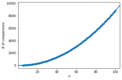
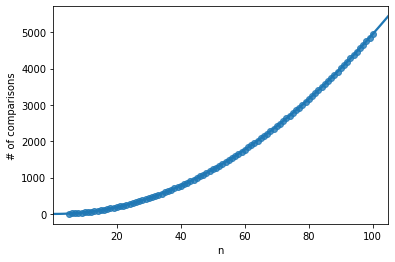
The following graph illustrates the time complexity. For each length of list from 5 to 100, I run 500 simulations on random lists, and count the number of comparisons required to finish the sorting. For example, n=60 is approximately 3000, which means that on average, a list of length 60 required 3000 comparisons from start to finish.
The line is a 2nd order polynomial approximation. Here we can see that it is a very good fit, reassuring us that the time complexity of the average case scenario is indeed O(n2).
Improvements
Notice how after each pass, the latgest i elements are already sorted into the correct locations. We can make use of this observation to improve the implemented algorithm, so that within each subsequent pass, we make fewer and fewer comparisons, since the last few elements are guaranteed to be in the correct order.
Selection Sort
 |
|---|
| (gif Credit) |
Unlike Bubble sort, which performs a series of immediate swaps, Selection sort finds (and selects) the minimal element from an unsorted list, and puts that selected element in order.
Python Implementation
# selection sort
def selection_sort(to_sort):
    """
    Given a list of integers,
    sorts it into ascending order with Selection Sort
    (done in place)
    and returns the sorted list
    """
    # length of array to sort
    list_len = len(to_sort)
    # for each pass, find the smallest element
    # and exchange it with the element at the index lcoation
    for i in range(list_len):
        # keep track of the index of the minimal element
        min_ind = i
        for j in range(i, list_len):
            # for all unsorted part of the list
            # do the pairwise comparisons
            if to_sort[j] < to_sort[min_ind]:
                # if new element is smaller, update min_ind
                min_ind = j
        # at the end of each pass
        # exchange the selected minimal element
        to_sort[i], to_sort[min_ind] = to_sort[min_ind], to_sort[i]

    return to_sort
Now let’s test the code:
# generate some random integers
import random
to_sort = random.sample(range(1, 1000), 20)

to_sort
# [991, 492, 629, 722, 856, 282, 735, 890, 548, 32, 124, 199, 546, 724, 234, 21, 728, 701, 333, 440]

selection_sort(to_sort)
# [21, 32, 124, 199, 234, 282, 333, 440, 492, 546, 548, 629, 701, 722, 724, 728, 735, 856, 890, 991]
Time Complexity
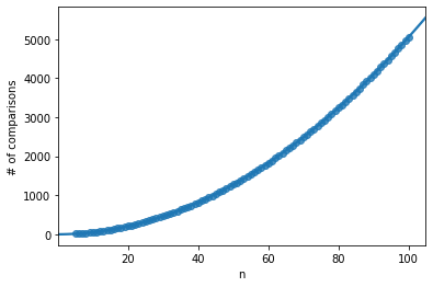
For Selection Sort, there is always the two nested loops to be performed, with the outer loop being the n passes, and the inner loop being the n-i comparisons within each pass. Therefore, for all cases, we have big-O complexity of O(n2).
Similarly to the simulation ran above for Bubble sort, here we can see that the 2nd order polynomial approximation is a very good fit for our time complexity, reassuring us that the time complexity of the average case scenario is indeed O(n2).
Insertion Sort
 |
|---|
| (gif Credit) |
An easy way to understand insertion sort is to think of how (most) sort playing cards, as the cards are being dealt one by one. For example, you have a deck of 5 cards, and you have already sorted them as you got them. Now you are dealt a sixth card. How do you maintain the sorted order? You insert the new card into the existing cards, to the correct location where it belongs.
Python Implementation
# insertion sort
def insertion_sort(to_sort):
    """
    Given a list of integers,
    sorts it into ascending order with Insertion Sort
    (done in place)
    and returns the sorted list
    """
    # length of array to sort
    list_len = len(to_sort)
    # for each pass, the elements to its left
    # is already sorted, and we need to insert
    # element i into the correct location
    for i in range(1, list_len):
        # element in question
        el = to_sort[i]
        # keep track of where to insert el
        shift_count = 0
        # start comparing from right to left
        # so that we can easily replace in place
        for j in range(i-1, -1, -1):
            if to_sort[j] > el:
                # for all elements larger than el
                # shift it 1 index to the right
                to_sort[j+1] = to_sort[j]
                # el needs to shift 1 more unit to the left
                shift_count += 1
            else:
                # once we hit an element not larger than el
                # we can terminate the process, since the rest
                # is all going to be smaller
                break
        # insert el
        to_sort[i-shift_count] = el

    return to_sort
Now let’s test the code:
# generate some random integers
import random
to_sort = random.sample(range(1, 1000), 20)

to_sort
# [806, 202, 383, 519, 592, 511, 96, 971, 133, 204, 587, 26, 760, 361, 582, 373, 661, 182, 744, 36]

insertion_sort(to_sort)
# [26, 36, 96, 133, 182, 202, 204, 361, 373, 383, 511, 519, 582, 587, 592, 661, 744, 760, 806, 971]
Time Complexity
Very similar to Selection Sort, we also have two nested loops here, each growing linearly as n grows, resulting in an overall O(n2). However, in the best case scenario, where we have an already sorted list, the inner loop will always terminate on first comparison, essentially reducing the runtime to the outer loop, which is simply n. Keep this feature in mind, as we will see in Part 2, how we would like to take advantage of this feature to construct a hybrid sorting algorithm called Tim Sort, where insertion sort is used to perform sortings on smaller lists, since consecutive ordered elements are often observed in real-world data.
If you are feeling comfortable with the basic sortings we have covered here, please move on to our Part 2 of the series, Sorting Algorithms w/ Python (Part 2), where we will see how we can improve our time complexity so that we could sort more efficiently on larger lists.

Leave a comment