

Algorithms with Python - Merge Sort and Tim Sort
Overview
Continuing on our journey to explore sorting algorithms with Python, we will talk about the following in our Part 2 of the Sorting Algorithms w/ Python series.
- Merge Sort
- Tim Sort
Links to Other Parts of Series
Array Sorting Complexities
Recall the time complexities (for a full summary, see Part 1).
| Algorithm | Time Complexity | ||
|---|---|---|---|
| Best | Average | Worst | |
| Merge Sort | Ω(nlog(n)) | θ(nlog(n)) | O(nlog(n)) |
| Tim Sort | Ω(n) | θ(nlog(n)) | O(nlog(n)) |
Note that compared to the algorithms we’ve talked about in Part 1, these algorithms has better time complexity properties. We will explain how that is achieved.
Sorting Algorithms
Merge Sort
 |
|---|
| (gif Credit) |
Merge sort is a classic “divide and conquer” algorithm, where we split up the list that needs to be sorted, sort them in small batches, then put them back together in order. In particular, the first step is to divide all elements into single elements, then combine into pairs, sort the pair, then combine into 4-element batches, and so on, until we have a sorted list.
Python Implementation
# merge sort
def merge_sort(to_sort):
    """
    Given a list of integers,
    sorts it into ascending order with Merge Sort
    (in place)
    and returns the sorted list
    """
    # length of array to sort
    list_len = len(to_sort)
    if list_len > 1:
        mid = list_len // 2
        L = to_sort[:mid]
        R = to_sort[mid:]

        # here we recursively incur the mergesort function
        # The effect is that it will first divide up the
        # entire list into individual bits.
        # Notice that merge_sort(single element) does nothing
        # so that when we reach merge_sort of 2 elements
        # we can finally go beyond this point
        merge_sort(L)
        merge_sort(R)

        # Once all elements are divided through the recursive calls
        # The function call can finally reach these later codes

        # i: index of element we are looking at in list L
        # j: index of element we are looking at in list R
        # k: total comparisons made / elements saved into arr
        i = j = k = 0

        # now we look at each list L and R
        # starting from the smaller elements (left)
        while i < len(L) and j < len(R):
            # if element from L is smaller than
            # element from R, we pop off the element from L
            # save it to our array
            # and move on to the next element in L
            if L[i] < R[j]:
                to_sort[k] = L[i]
                i += 1
            # similarly the case if the element in R is larger
            else:
                to_sort[k] = R[j]
                j += 1

            k += 1

        # Checking if any element was left
        # when one of the list L or R has been exhausted
        # If so, all elements left are larger than the rest.

        # if i < len(L): R is exhausted.
        # save all remaining elements from L into arr
        while i < len(L):
            to_sort[k] = L[i]
            i += 1
            k += 1

        # similarly the opposite case
        while j < len(R):
            to_sort[k] = R[j]
            j += 1
            k += 1

    return to_sort
Now let’s test the code:
# generate some random integers
import random
to_sort = random.sample(range(1, 1000), 20)

to_sort
# [61, 309, 414, 688, 123, 669, 473, 845, 330, 231, 173, 758, 797, 374, 511, 20, 28, 958, 196, 25]

insertion_sort(to_sort)
# [20, 25, 28, 61, 123, 173, 196, 231, 309, 330, 374, 414, 473, 511, 669, 688, 758, 797, 845, 958]
Time Complexity
Regardless of the initial condition of the list, Merge Sort always divide and conquers. Within each level of division, the number of comparisons required is on the order of n (n/2 for last level, n/2 to 3n/4 for second to last level, etc.), and the number of levels are of order log(n), since 2# of levels is on the order of n. To show how stark the difference this is from the quadratic time complexities, the # of comparisons is plotted below for merge sort and insertion sort:
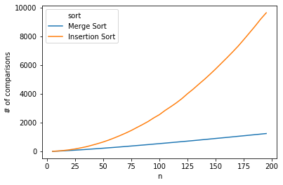
As we can see, as the length of the list increases, the big-O difference really starts to reveal itself, where the # of comparisons required for insertion sort simply takes off.
Tim Sort
Tim sort was created in 2001 for implementations of sorting functionalities in Python. It is real-world focused, takes advantage of the superior performance of insertion sort on smaller lists in real-world data where consecutive ordered elements are often present, and the ability of merge sort to combine sorted sub-lists into one final sorted list. The actual implementation has more details, but the implementation below should give us a feel of the inner workings.
Python Implementation
# tim sort
# Adapted from https://gist.github.com/nandajavarma/a3a6b62f34e74ec4c31674934327bbd3

# custom binary search
def binary_search(arr, item, start, end):
    """
    This is a recursive implementation of
    searching for the correct position of an `item`
    in a sorted array `arr`
    using binary search technique.

    The item may or may not be present in arr.

    start / end are specified for recursive calls.

    Initial call would specify them as start / end of
    arr, respectively. i.e.
    start = 0
    end = len(arr) - 1
    """

    # first specify end game
    # if the two pointers meet,
    # it means we are done searching.
    # and we need to determine the final index
    if start == end:
        if arr[start] > item:
            # item should be inserted to the left of start
            return start
        else:
            # item should be inserted to the right of start
            return start + 1
    # if we arrive at this state without finding the location
    # ((start + end) // 2 is within 1 of end)
    # and start != end --> start == end - 1
    # it means that start is the correct location
    if start > end:
        return start

    mid = (start + end) // 2
    # if item is larger, search in upper half
    if arr[mid] < item:
        return binary_search(arr, item, mid + 1, end)
    # else, search in lower half
    elif arr[mid] > item:
        return binary_search(arr, item, start, mid - 1)
    else:
        return mid

# insertion part
def insertion_sort(to_sort):
    """
    Given a list of integers,
    sorts it into ascending order with Insertion Sort
    (done in place)
    and returns the sorted list
    """
    # length of array to sort
    list_len = len(to_sort)
    # for each pass, the elements to its left
    # is already sorted, and we need to insert
    # element i into the correct location
    for i in range(1, list_len):
        # element in question
        el = to_sort[i]
        # keep track of where to insert el
        shift_count = 0
        # start comparing from right to left
        # so that we can easily replace in place
        for j in range(i-1, -1, -1):
            if to_sort[j] > el:
                # for all elements larger than el
                # shift it 1 index to the right
                to_sort[j+1] = to_sort[j]
                # el needs to shift 1 more unit to the left
                shift_count += 1
            else:
                # once we hit an element not larger than el
                # we can terminate the process, since the rest
                # is all going to be smaller
                break
        # insert el
        to_sort[i-shift_count] = el

    return to_sort

def merge(left, right):
    """
    Takes two sorted lists and returns a single sorted list by comparing the
    elements one at a time.

    For detailed explanation of the logic, see Part 1
    where merge_sort is explained and implemented
    """
    if not left:
        return right
    if not right:
        return left
    if left[0] < right[0]:
        return [left[0]] + merge(left[1:], right)
    return [right[0]] + merge(left, right[1:])

# putting together
def timsort(to_sort):
    # timsort uses a concept called "runs"
    # where consecutive elements in order will be
    # put into a run and merged together.
    # The actual timsort is more advacned in constructing the
    # runs, but the code below suffices to illustrate the logic.
    runs, sorted_runs = [], []
    l = len(to_sort)
    new_run = [to_sort[0]]
    for i in range(1, l):
        # if last element
        if i == l-1:
            # append to new run, and add new run to all runs
            new_run.append(to_sort[i])
            runs.append(new_run)
            break
        # if next element is larger then current
        # i.e. is not in order
        if to_sort[i] < to_sort[i-1]:
            # if current run is empty
            if not new_run:
                # append a singleton list to the runs
                # and append next element to new run
                runs.append([to_sort[i-1]])
                new_run.append(to_sort[i])
            # if we have a non-empty run
            else:
                # append the run to the list of runs
                runs.append(new_run)
                # start new empty run
                new_run = []
        # if in order, just add next element to current run
        else:
            new_run.append(to_sort[i])

    # Note that our implementation of the "runs"
    # actually results in already sorted runs
    # such that this insertion_sort step is redeundant.
    # However, in a more sophisticated setup, the "runs"
    # would not be completey sorted, but would comtain
    # some bits of unsorted data, and truncated to make sure
    # each run is of specified length (or shorter),
    # where insertion sort performs best
    for each in runs:
        # use insertion sort to sort each run,
        # and append to sorted_runs to keep track
        sorted_runs.append(insertion_sort(each))
    sorted_array = []
    for run in sorted_runs:
        # finally, for each of these sorted runs
        # we merge them together
        sorted_array = merge(sorted_array, run)
    return sorted_array
Time Complexity
In best case scenario, where the list is already sorted, the run-construction, insertion sort, and merging part each takes linear time. Hence a big-) of n. Average case and worst case is bounded by merge sort’s nlog(n) complexity.

Leave a comment