

XGBoost - AdaBoost
Links to Other Parts of Series
Prerequisites
Overview
If you’re not familiar with Decision Trees and Random Forests, and haven’t already checked out the blog posts linked above, please check that out first before proceeding with this post on AdaBoost, since this does build upon the former two.
Now that we got that covered, let’s dive right in!
Note: This post is heavily based on this awesome open course lecture from MIT: 6.034 Recitation 10: Boosting (Adaboost), which I would recommend you checking out (in fact, the entire series is quite fascinating).
What is AdaBoost?
AdaBoost stands for Adaptive Boosting. Just like Random Forest, AdaBoost is also a type of ensemble learning algorithm, which uses and combine multiple “weaker” learning algorithms and convert them into a potentially better abd stronger learning algorithm. The differences, however, are plenty. For example, in our Random Forest model, each decision tree in the model essentially holds the same weight. In comparison, our AdaBoost model will assign different weights (voting power) adaptively through the iterative process. Let’s get into more detail!
Steps
The goal is to construct an ensemble learning algorithm H(x) = f(a_1 * h_1(x) + a_2 * h_2(x) + ...) where a_i’s are the voting power (weights of each weak learner) , and h_i’s are the weak learners selected to make up out ensemble model.
0. Set of Weak Classifiers
To construct an ensemble model, we first need a set of weak classifiers to select from. For AdaBoost, we often times will use 1-level Decision Trees, or so-called stumps, as the weak learners. Now that we have the groundwork laid out, we can start talking about the important steps in AdaBoost.
1. Weight Initialization
An important aspect of the “adaptiveness” of AdaBoost is that it can shift its focus onto specific samples as the models gets trained. This is done by taking into consideration the weights of each sample. However, at the very beginning, we might not have any reasons to focus on any spoecific samples, so the initialization is usually a uniform weight.
2. Calculate Error Rate
For each weak learner, we calculate its error rate by adding up all the weights of the samples it has misclassified.
3. Pick the best weak learner
Once we have the error rates for each weak learner, we will pick the one with the smallest error rate (note: we might pick the one with the error rate farthest away from 1/2, since always making the wrong prediction can be adapted to always make the correct prediction. But for simplicity, we simply look at the smallest error rate for now).
4. Calculate Voting Power
Now we have the h_i part, and we need to decide on the corresponding a_i. There are a couple ways to do this, but following the linked lecture, we will stick to the following formula: a_i = 0.5 * Ln((1-e_i)/e_i). That is, we will take the natural log of the ratio of (1-the error rate) and (the error rate), and multiply it by point 5. Notice that this formula returns 0 if we have an error rate of 0.5 - if we are no better than randomly guessing, we don’t give you any say in the vote. Also notice that if e_i is larger than 0.5, so we are more often incorrect than right, we may assign it a negative voting power. This is exactly the case we have mentione earlier, that a very high error rate could also be quite informative to us as long as we adapt it appropriately.
5. Finished?
Now we need to decide our terminating condition. We can specify: 1. We want to find at most 4 h_i’s; 2. We want to continue the process until the ensemble H reaches a certain performance criteria; 3. We stop when there is no more good h’s left. Regardless of how we decide on this, if we continue, then our next step would be …
6. Update the Weights (of the sample data)
Up to now, all samples have the same weights (by construction / initialization). If we continue on, we would like to focus a bit more on the samples that we were not able to correctly classify. Therefore, we come up with this updating formula:
w_new = w_old / (2*(1-e_i)) if correctly classified;
w_new = w_old / (2*e_i) if incorrectly classified;
Note a couple of interesting facts:
- Since e_i = sum of all w_old of misclassified, sum of all w_new of misclassified = sum of all
w_old / (2*e_i)of misclassified =e_i / (2*e_i)= 1/2; - Similarly, sum of all w_new of correctly classified samples is also one-half;
- When error rate (e_i) is less than 1/2 (not considering always wrong cases),
(2*e_i) < 1, and hence incorrectly classfied samples will have a larger weight in the next round, making the model focus more on the incorrectly classified samples.
7. Repeat!
Now with the new weights, we go back to Step 2 and repeat the process, appending new weak learners h to the ensemble H along the way, until we determine it is good to stop, as described in Step 5.
An Example
To get things started, let’s consider the following example.
|
|---|
| (source: Example taken from 6.034 Recitation 10: Boosting (Adaboost)) |
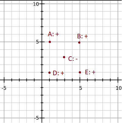
Here we have 5 points, A to E, where all points except C shall be classified as “+”. We now consider the following classifiers:
L1: x < 2
L2: x < 4
L3: x < 6
L4: x > 2
L5: x > 4
L6: x > 6
where each classifier will classify an sample data to be of class “+” if it fits the criterion. Hence, we have the following predictions:
L1: x < 2 : A,D | B,C,E
L2: x < 4 : A,C,D | B,E
L3: x < 6 : A,B,C,D,E | NULL
L4: x > 2 : B,C,E | A,D
L5: x > 4 : B,E | A,C,D
L6: x > 6 : NULL | A,B,C,D,E
resulting in the following misclassifications:
L1: x < 2 : A,D | B,C,E  : INCORRECT: B,E
L2: x < 4 : A,C,D | B,E : INCORRECT: C,B,E
L3: x < 6 : A,B,C,D,E | NULL : INCORRECT: C
L4: x > 2 : B,C,E | A,D : INCORRECT: A,C,D
L5: x > 4 : B,E | A,C,D : INCORRECT: A,D
L6: x > 6 : NULL | A,B,C,D,E : INCORRECT: A,B,D,E
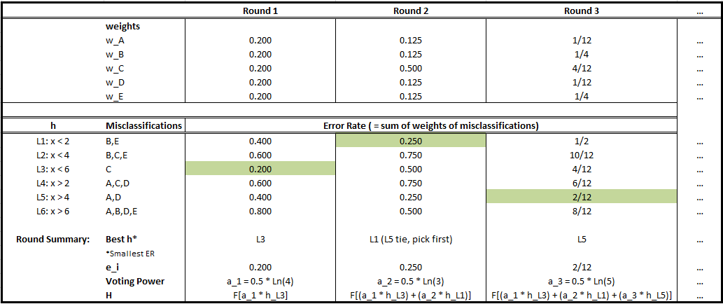
Walk through the steps:
Round 1
- Initialize weights to be 1/5 for all.
- Error rates: We add up the weights of the misclassified samples for each weak learners;
- We pick the weak learner with the smallest error rate (L3);
- We calculate the voting power according to our formula;
- We append this component to our ensemble, and update the weights for our samples;
- We continue to next round.
Round 2
- Given the updated weights, we calculate new error rates;
- …… Iterate the process, shown in the chart below.
|
|---|
| (source: Example taken from 6.034 Recitation 10: Boosting (Adaboost)) |
Conclusion
Building on random forest, we have made our forest adaptive on previous results, focusing on hard to classify samples in later rounds. By choosing hyperparameters wisely, such as termination conditions, we can often address overfitting issues as well. All said, AdaBoost is one of the algorithms that work decently right out-of-the-box, and it is important to understand the concepts for our later blog posts on Gradient Boosting and the finale - XGBoost.

Leave a comment