XGBoost - Decision Trees

Links to Other Parts of Series

• Machine Learning Series

Overview

In this first section of our Machine Learning series, we will talk about a popular machine learning technique for regression and classification problems, namely XGBoost. As usual, we will start from the basics, and start building towards the fully featured model. The concepts we will cover in a series of posts are:

1. Decision Tree;
2. Random Forest;
3. AdaBoost;
4. Gradient Boost;
5. XGBoost!

We will cover each topic with a varying level of depth, but should suffice to get us towards to main goal here: Understanding and successfully implementing XGBoost models! We will start off this series with our first post talking about …

Decision Trees!!

What is a Decision Tree?

In Machine Learning, a Decision Tree (DT) is a simple yet effective predictive model that can be utilized for both regression models (when the target value is continuous) and classification problems (discrete targets). The former is often referred to as a Regression Tree, while the latter a Classifcation Tree. An example for a Classification Tree would be to predict whether a person obtaining a loan will defaut or not, while a Regression Tree might be to predict the Credit score of that person.

Decision Trees are easy to visualize and understand. Take the following graph as an example:

(source: Decision Tree Classification)

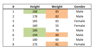
Here we can imagine we have a dataset of people with 3 attributes: height, weight and gender, and we are trying to predict the gender of a person based on height and weight. Don’t mind the over-simplifications here, we are just trying to grasp the idea. The DT first splits up our dataset by asking if the person’s height is over 180cm, and classify the person as a male if the answer is “yes”. For those with a “No”, we will further ask about the person’s weight, and if the person is heavier than 80kg, the model outputs “male”, while classifying the person as a “female” otherwise.

We will learn how to deal with different types of inputs (continuous such as height / weight, discrete such as ethnicity, and so on), how to pick the best threshold / criteria (“180cm” / “80kg”), how to decide whether to split first on “height” (as we do here), or to first split on “weight”. But before all that, some simple terminology would be helpful:

(source: What are Decision Trees?)

We call the initial state the “root node”, and all other nodes that has a child node “interior nodes”. Those that do not have a child node, are called “leaf nodes”, and those are where the final predictions are made.

How do we choose the order of inputs to split on?

Continuing to use our height / weight example, and say we take the thresholds as given (so we don’t need to worry about choosing a different threshold). Then how do we dicide whether to split on height first, or weight first? The usual technique involves a metrics called “Gini impurity index”.

Gini Impurity

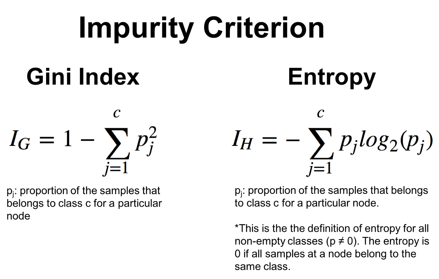
Recall that when we do a split, we will split the input data into 2 sets: those we answer “yes” to, and those with a “no”. Within each set, we calculate the proportion of samples that is of a particular target characteristic - here, “male” and “female”. Then for these calculated ratios, we substract the sum of their squared value from 1. Concretely, the formula is shown below.

(source: What is difference between Gini Impurity and Entropy in Decision Tree?)

As we can see - Entropy could be another criterion, but we will not get into that here. The formula on the left shows how we calculate a Gini Index / Impurity. Now let’s take a made-up dataset and try to perform this exercise.

Let’s say we split on Height > 180 - what is the Gini Index? The first set is those who are under 180. Within this set, we calculate the Gini index as: 1 - (2/5)^2 - (3/5)^2 = 12/25. For the set with people over 180, the Gini index is similarly calculated as 1 - (3/3)^2 - (0/3)^2 = 0. Explanation: For those under 180, we have a total of 5 samples, and 2 of them are male, while 3 of them are female. For those over 180, all 3 samples are male, and the Gini is exactly 0 - we have no impurity since all samples in this set is Male.

Now, to get the Gini Impurity for using “height > 180” to spli patients, is a weighted average of the child node’s gini imprutiy: 5/8 * 12/25 + 3/8 * 0 = 0.3. Explanation: Total of 8 samples, 5 in the first set (which has Gini impurity of 12/25), and 3 in the second set (with Gini 0).

Now let’s repeat the process for “weight > 80kg”. We first split the data set into 2 sets, and calculate the gini of each set.

Set 1 [“>80kg”]: Gini = 1 - (3/4)^2 - (1/4)^2 = 3/8

Set 2 [”<=80kg”]: Gini = 1 - (2/4)^2 - (2/4)^2 = 1/2

Gini for splitting on “80kg weight”: 4/8 * 3/8 + 4/8 * 1/2 = 7/16

Once we have these two Gini’s, we should pick the one with the lowe Gini Impurity to split on first. Intuitively, this allows us to subdivide the dataset in the cleanest manner, since it leads to the lowest “impurity”. Here, 7/16 > 0.3, so indeed, first splitting on Height makes sense!

How do we handle various types of inputs?

1. For simple Yes/No binary inputs, it is clear that we can simply split on the answers “yes”/”no”;
2. For ranked data, we calculate the impurity scores for each possible value (possibly in a less than or equal to form), and split on the value giving us the lowest Gini;
3. For continuous / numeric data, we can treat it similarly to ranked data, but we usually sort our data and test the mid-points between each existing values. For our heigh / weight example, we might have tested 162.5 (mid between 160 and 165), and various other points - and ended up with 180 (probably not true for our example data set);
4. For multiple choice data, we usually calculate the Gini’s for various ways of splitting the data. For example, if we have categories A, B, C, and D, we can split it into A vs Others, A or C vs Others, etc. Then we choose the split that results in the lowest Gini!

Sounds a bit complicated, or at least a bit tedious, to implement? Thankfully, most statistical packages will handle these works for you, but knowing what it’s doing behind the scenes is still critical to effectively applying these models!

Python Time!

Let’s put our hands on some real code, and see how we can implement a simple program with our newly learned knowledge. Comments in the code should walk you through what we’re trying to do.

# first construct a simple dataset
# with rules:
# male are of height ~185 +- 10, weight ~85+-10
# female are of height ~175 +- 10, weight ~75+-10

import pandas as pd
import random

data = []
for i in range(1000):
    if random.random() > 0.5:
        # generate a male
        gender = 'male'
        height = 185 + random.randint(-10, 10)
        weight = 85 + random.randint(-10, 10)
    else:
        # generate a female
        gender = 'female'
        height = 175 + random.randint(-10, 10)
        weight = 75 + random.randint(-10, 10)
    data.append({
        'height': height,
        'weight': weight,
        'gender': gender
    })

df = pd.DataFrame(data)

# use sklearn's DecisionTree Classifier
from sklearn import tree

X = df[['height', 'weight']]
Y = df['gender']

# Here we specify depth=2 since if we don't do it
# it will try to split it into many very fine categories
# (to make "best" predictions):
#
# The maximum depth of the tree.
# If None, then nodes are expanded until all leaves are pure or
# until all leaves contain less than min_samples_split samples.

clf = tree.DecisionTreeClassifier(max_depth=2)
clf = clf.fit(X, Y)

# To visualize our tree
dot_data = tree.export_graphviz(clf, out_file='sample_output.dot')

# Then go to a website such as http://webgraphviz.com/ and
# paste in the sample_output.dot
# Or install a visualization software such as graphviz
# and do it in python

Result

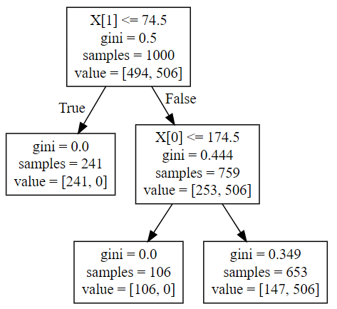
As we can see, the classifier first decided to split on the criterion “weight < 74.5”, since that results in all females in one set (impurity = 0), and some mix in the other set. This first subset becomes a leaf node, since it is pure now. Within that other set, the algorithm found “height <= 174.5” to be a good criterion, since all those above are indeed “male” by construction.

Conclusion

We have seen how this simple method can be used to analyze datasets, and effectively find the determining factors that can help classify a sample. A common criticism of such approach is that it usualyl performs very well on sample sets, but not as well on new data prediction. To overcome this pitfall, and to move towards a fully fledged XGBoost model, we will next cover Random Forest Models - yes, it’s exactly what it sounds - a forest made up of many decision trees, and some randomness involved!

Resources