

XGBoost - XGBoost Code Example
Links to Other Parts of Series
Prerequisites
Overview
If you’re not familiar with the contents linked above, please check those out first before proceeding with this post on XGBoost’s coding example, since having at least some understanding of what it is doing underneath the hood would really benefit your learning experience in going over this example.
Now that we got that covered, let’s dive right in!
The IMDB Challenge
We will use XGBoost to explore the Box Office prediction challenge offered on Kaggle, TMDB Box Office Prediction. From the official description:
In this competition, you’re presented with metadata on over 7,000 past films from The Movie Database to try and predict their overall worldwide box office revenue. Data points provided include cast, crew, plot keywords, budget, posters, release dates, languages, production companies, and countries. You can collect other publicly available data to use in your model predictions, but in the spirit of this competition, use only data that would have been available before a movie’s release.
Our Demo Version
This demo will mostly draw on this kaggle notebook by Kamal Chhirang, but quite heavily dumbed down (and extended in other ways) so that we can focus on XGBoost here. We will not use the external datasets (neither the extra features, or the additional rows of training data) some others are using. We will not even try to make use of all the standard data, as some preprocessing would take too long to explain and lay out clearly Instead, we will use the most basic features, but features of different types: continuous features such as Budget, and categorical ones such as Genres.
Code!!
Set Up
You would need to download the dataset from the Kaggle page, and install some python packages commonly used in such data science / machine learning tasks, such as numpy, pandas, scikit-learn, but most importantly for us, xgboost!
import numpy as np
import pandas as pd
import matplotlib.pyplot as plt
import seaborn as sns
import warnings
from tqdm import tqdm
from datetime import datetime
import json
from sklearn.preprocessing import LabelEncoder

# set paths
import os
ROOT = 'E:\\2_github_projects\\kaggle-imdb'
DATA_PATH = os.path.join(ROOT, 'data')

TRAINING_PATH = os.path.join(DATA_PATH, 'train.csv')
TESTING_PATH = os.path.join(DATA_PATH, 'test.csv')
Some Exploration
First we do some basic data exploring - see the original notebook linked above for more exploration. We will only glance through some more interesting ones, then go right into the model part.
Basic Info
We see there are 3000 training examples available to us, with a variety of features.
train = pd.read_csv(TRAINING_PATH)
train.info()

<class 'pandas.core.frame.DataFrame'>
RangeIndex: 3000 entries, 0 to 2999
Data columns (total 23 columns):
id                       3000 non-null int64
belongs_to_collection    604 non-null object
budget                   3000 non-null int64
genres                   2993 non-null object
homepage                 946 non-null object
imdb_id                  3000 non-null object
original_language        3000 non-null object
original_title           3000 non-null object
overview                 2992 non-null object
popularity               3000 non-null float64
poster_path              2999 non-null object
production_companies     2844 non-null object
production_countries     2945 non-null object
release_date             3000 non-null object
runtime                  2998 non-null float64
spoken_languages         2980 non-null object
status                   3000 non-null object
tagline                  2403 non-null object
title                    3000 non-null object
Keywords                 2724 non-null object
cast                     2987 non-null object
crew                     2984 non-null object
revenue                  3000 non-null int64
dtypes: float64(2), int64(3), object(18)
memory usage: 539.2+ KB
We can further use train.head() to look at some real data. Here we have discovered that things like spoken_languages, Keywords, Genres and more categorical values are stored in a dictionary-like format. This will affect how we preprocess our data later on.
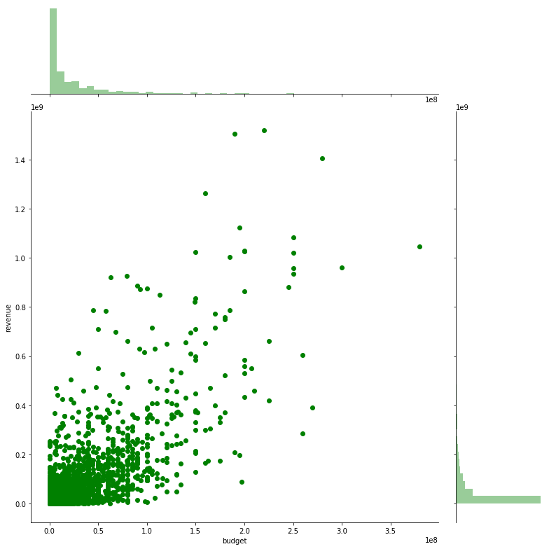
Budget - Revenue Relation
sns.jointplot(x="budget", y="revenue", data=train, height=11, ratio=4, color="g")
plt.show()
|
|---|
We see that most films have budget clustered around the origin (low budget / low revenue), but on a high level, most points do follow the diagonal, meaning a higher budget could lead to a higher revenue. However, there are a lot of variations.
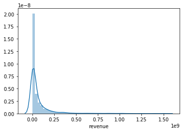
Revenue Distribution
sns.distplot(train.revenue)
|
|---|
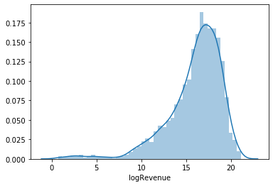
We see that revenue is highly skewed, and in light of this, we might consider training on the log-revenues:
train['logRevenue'] = np.log1p(train['revenue'])
sns.distplot(train['logRevenue'] )
|
|---|
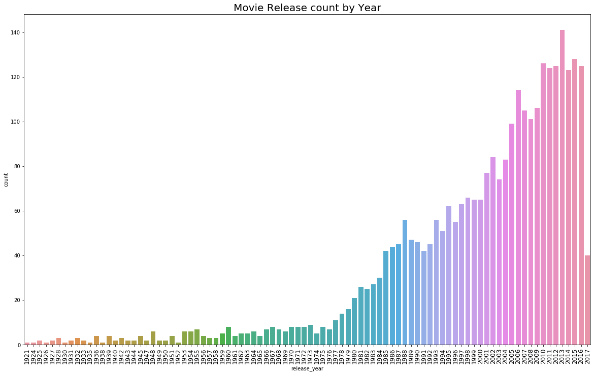
Movies Count by Year
Let’s see which years our movies in the training set was made in!
# First we need to parse the "release_date" given to us
train[['release_month', 'release_day', 'release_year']] \
    = train['release_date'].str.split('/', expand=True).replace(np.nan, -1).astype(int)

# Some rows have 4 digits of year instead of 2, that's why
# I [ORIGINAL AUTHOR] am applying (train['release_year'] < 100) this condition
train.loc[ (train['release_year'] <= 19) & (train['release_year'] < 100), "release_year"] += 2000
train.loc[ (train['release_year'] > 19)  & (train['release_year'] < 100), "release_year"] += 1900

releaseDate = pd.to_datetime(train['release_date'])
train['release_dayofweek'] = releaseDate.dt.dayofweek
train['release_quarter'] = releaseDate.dt.quarter

# Now we can plot it

plt.figure(figsize=(20, 12))
sns.countplot(train['release_year'].sort_values())
plt.title("Movie Release count by Year", fontsize=20)
loc, labels = plt.xticks()
plt.xticks(fontsize=12, rotation=90)
plt.show()
|
|---|
XGBoost Model
Now let’s get into the model implementation. The original author implemented 3 models (one of which is XGBoost), and implemented K- cross-validation. I will simply do an XGBoost model since that is our focus, and will not worry too much about the cross-validating.
Preprocessing
train = pd.read_csv(TRAINING_PATH)

# get target for training - notice the log-tranformation
train['revenue'] = np.log1p(train['revenue'])
y = train['revenue'].values


# we stream-line the preprocessing into a function
# so that it is easier to repeat,
# but most importantly, if we were actually using the test set
# this would make sure our training and testing set have the same format
def pre_process(df):

    # This is the release date formatting we have seen above
    df[['release_month', 'release_day', 'release_year']] = \
        df['release_date'].str.split('/', expand=True).replace(np.nan, -1).astype(int)
    # Some rows have 4 digits of year instead of 2, that's why I am applying (train['release_year'] < 100) this condition
    df.loc[ (train['release_year'] <= 19) & (df['release_year'] < 100), "release_year"] += 2000
    df.loc[ (train['release_year'] > 19)  & (df['release_year'] < 100), "release_year"] += 1900

    releaseDate = pd.to_datetime(df['release_date'])
    df['release_dayofweek'] = releaseDate.dt.dayofweek
    df['release_quarter'] = releaseDate.dt.quarter

    # this function is used to extract values from
    # the dictionary-like structures used to store
    # categorical features
    def get_dictionary(s):
        try:
            d = eval(s)
        except:
            d = {}
        return d

    # Among them we will only use the "genres" feature
    for col in ['genres']:
        df[col] = df[col].map(lambda x:
                    sorted([d['name'] for d in get_dictionary(x)])
                ).map(lambda x: ','.join(map(str, x)))

        temp = df[col].str.get_dummies(sep=',')
        # temp is a df here with indicator columns
        # each genre is transformed into a column, with 0s and 1s
        # to indicate if the film in the row is of this genre
        df = pd.concat([df, temp], axis=1, sort=False)

    # drop a bunch of cols
    df = df.drop([
            'id', 'belongs_to_collection', 'genres', 'homepage',
            'imdb_id', 'overview', 'runtime', 'poster_path',
            'production_companies', 'production_countries', 'release_date',
            'spoken_languages', 'status', 'title', 'Keywords', 'cast',
            'crew', 'original_language', 'original_title', 'tagline'
        ], axis=1)

    # if training set, also drop revenue
    # testing set does not have this col
    if 'revenue' in df.columns:
        df = df.drop(['revenue'], axis=1)

    return df


train = pre_process(train)

#### Not using this here ####
# but if we do want to use the test set with XGBoost
# we need to make sure the columns are the same
# (including the order of the columns!)
# add TV Movie to test - since it is in training
test['TV Movie'] = 0
# then reorder as in training
test = test[train.columns]
Training
import xgboost as xgb

train = pd.read_csv(TRAINING_PATH)
train = pre_process(train)
# we wil leave out 500 (out of 3000) to be as validation set
trn_x = train[:-500]
trn_y = y[:-500]
val_x = train[-500:]
val_y = y[-500:]


# here we specify some parameters for our XGBoost model
params = {
    'objective': 'reg:linear',
    'eta': 0.01,
    'max_depth': 10,
    'subsample': 0.6,
    'colsample_bytree': 0.7,
    'eval_metric': 'rmse',
    'silent': True,
    }

model = xgb.train(
            params,
            xgb.DMatrix(trn_x, trn_y),
            100000,
            [(xgb.DMatrix(trn_x, trn_y), 'train'), (xgb.DMatrix(val_x, val_y), 'valid')],
            verbose_eval=1,
            early_stopping_rounds=500
            )
100000 is the boosting round we have specified, but we have also specified “early_stopping_rounds”, which would stop the training if validation metric is no longer improving in the specified rounds (So no, we will most likely NOT go full 100000 rounds!). xgb.DMatrix(trn_x, trn_y), is the data to be trained on.
Now let’s look at the params (consulting the documentation):
objective: Specifies the learning task and the corresponding learning objective. “reg:linear” –linear regression, which is what we use to make the prediction of (log) revenue;eval_metric: The metric used for evaluation. For linear regression (and this Kaggle Challenge’s specification), we will use “rmse”: root mean square error;eta: Step size shrinkage used in update to prevents overfitting. After each boosting step, we can directly get the weights of new features. and eta actually shrinks the feature weights to make the boosting process more conservative;max_depth: The maximum depth of a tree being constructed;subsample: Subsample ratio of the training instance. Setting it to 0.5 means that XGBoost randomly collected half of the data instances to grow trees and this will prevent overfitting. Recall Random Forest where we have discussed this.colsample_bytree: Similar to above, but randomly selecting features. Also used to reduce overfitting.silent: 0 means printing running messages, 1 means silent mode.
Now we run the training, and get the following result:
[0] train-rmse:15.5907  valid-rmse:15.7074
Multiple eval metrics have been passed: 'valid-rmse' will be used for early stopping.

Will train until valid-rmse hasn't improved in 500 rounds.
[1] train-rmse:15.4394  valid-rmse:15.5549
[2] train-rmse:15.2897  valid-rmse:15.4056
[3] train-rmse:15.141   valid-rmse:15.2555
[4] train-rmse:14.9937  valid-rmse:15.1071
[5] train-rmse:14.848   valid-rmse:14.9606
[6] train-rmse:14.7039  valid-rmse:14.8152

...
...
...
...

[1066]  train-rmse:0.450771 valid-rmse:1.9841
[1067]  train-rmse:0.449782 valid-rmse:1.98419
[1068]  train-rmse:0.448869 valid-rmse:1.98398
[1069]  train-rmse:0.448372 valid-rmse:1.98406
[1070]  train-rmse:0.44772  valid-rmse:1.98413
Stopping. Best iteration:
[570]   train-rmse:0.91243  valid-rmse:1.95397
Making Predictions
For simplicity, we will use validation set to check out our model performance. If we use test set, we would have to actually go find the true value of the Box Offices… In validation set, we have that info already!
# val_x is the features for validations set
# we use model.predict to perform predictions on these features
val_pred = model.predict(xgb.DMatrix(val_x), ntree_limit=model.best_ntree_limit)

# read in training set again (since old training has been processed)
train = pd.read_csv(TRAINING_PATH)
# construct a new DataFrame to store some data we want
result_df = pd.DataFrame()
# for example - title of a film
# -500 is how we got the validation set
result_df['title'] = train[-500:]['title']
# recall that the model predicts log-revenue
# to transform back to regular revenue
# we need to to an exponential transformation
result_df['prediction'] = np.expm1(val_pred)
# val_y is the true value of the validation set
# we also need to transform it
# (or perhaps we could just read in train[-500:]['revenue'])
# should be about the same
result_df['true'] = np.expm1(val_y)

# sort in descending order
result_df.sort_values(by=['prediction'], inplace=True, ascending=False)

# these large numbers are hard to read
# let's do a little formatting
def format_value(val):
    if val > 10**9:
        return '{} {}'.format(round(val/10**9, 2), 'B')
    if val > 10**6:
        return '{} {}'.format(round(val/10**6, 2), 'M')
    if val > 10**3:
        return '{} {}'.format(round(val/10**6, 2), 'K')
    return val


result_df['index'] = np.arange(len(result_df))
# create new cols for formatted values - we still want to keep
# original values for plotting purposes
result_df['prediction_pretty'] = result_df['prediction'].apply(format_value)
result_df['true_pretty'] = result_df['true'].apply(format_value)
Now we are ready to check out the results!
print(result_df[['title', 'prediction_pretty', 'true_pretty']].to_string())

-->

                                                  title prediction_pretty true_pretty
2770                            Avengers: Age of Ultron          730.73 M      1.41 B
2532                  The Hobbit: An Unexpected Journey          701.93 M      1.02 B
2737                                            Spectre          612.45 M    880.67 M
2802            Harry Potter and the Chamber of Secrets          514.78 M    876.69 M
2858                                               Cars          465.75 M    461.98 M
2938                                         Prometheus          402.19 M    403.17 M
2647               Mission: Impossible - Ghost Protocol          401.13 M    694.71 M
2570                                  The Polar Express           398.6 M    305.88 M
2562                                       Finding Dory          351.75 M      1.03 B
2793                                              Ted 2           343.1 M    217.02 M
2739                                    The Incredibles          317.27 M    631.44 M
2623        Valerian and the City of a Thousand Planets          265.29 M     90.02 M
2927                                    Die Another Day          222.15 M    431.97 M
2866                 National Treasure: Book of Secrets          219.64 M    457.36 M
2518                      You Don't Mess with the Zohan          209.86 M     201.6 M
2663                             Paul Blart: Mall Cop 2          195.11 M     107.6 M
2729                                      The Boss Baby           182.1 M    498.81 M
2644                                  Starship Troopers          178.25 M    121.21 M
2899                                           Dinosaur          173.37 M    354.25 M
2738                          Atlantis: The Lost Empire          172.74 M    186.05 M
2880                                   White House Down          170.85 M    205.37 M
2603                                Alien: Resurrection          151.98 M     162.0 M
2895                                          The Score          151.39 M     71.07 M
2839                                  The Mask of Zorro          151.38 M    250.29 M
2547                                        I Am Legend           149.8 M    585.35 M
2993                                       The Terminal          143.57 M    219.42 M
2669                                         Pocahontas          139.21 M    346.08 M
2648                                     This Means War          135.44 M    156.97 M
2843              The Mortal Instruments: City of Bones          134.24 M     90.57 M
2846                                             Robots           132.4 M     260.7 M
2748                                          Rambo III          131.96 M    189.02 M
2834                             Something's Gotta Give          131.86 M    266.73 M
2514                                      The Equalizer          124.96 M    192.33 M
2631                                        Cloud Atlas          124.22 M    130.48 M
2606                                       Analyze This          123.31 M    176.89 M
2626                                               Doom          120.74 M     55.99 M
2541                                         This Is 40          120.36 M     88.06 M
2599                                 Enemy of the State          119.93 M    250.65 M
2709                                  The Scorpion King          119.44 M    165.33 M
2517                       Asterix at the Olympic Games          118.53 M     132.9 M
2935                                 The Stepford Wives          118.27 M     102.0 M
2943                          James and the Giant Peach          116.94 M     28.92 M
2740                              The Magnificent Seven          116.63 M    162.36 M
2719                                            Ben-Hur          116.03 M     94.06 M
2870                                    The Italian Job          115.89 M    176.07 M
2715                                 The Sweetest Thing          114.25 M      68.7 M
2530                                        The Kingdom          113.93 M     86.66 M
2558                                                  9          109.45 M     48.43 M
2997                            The Long Kiss Goodnight          104.94 M     89.46 M
2778                                   The Longest Yard          104.91 M    190.32 M
2984                                           S.W.A.T.          104.69 M    116.64 M
2632                                         Red Planet          102.88 M     33.46 M
2787                                    The Book of Eli          100.65 M    157.11 M
2773                                          The Siege          100.25 M    116.67 M
2911                            Exorcist: The Beginning          100.24 M      78.0 M
2643                                       Nim's Island           99.24 M    100.08 M
2782                                       Out of Sight           98.19 M     77.75 M
2777                                        The Phantom           94.51 M      17.3 M
2931                                         Titan A.E.           94.04 M     36.75 M
2734                                               Paul           91.52 M     97.55 M
2954                                              Alfie           90.96 M      13.4 M
2965                                     Les Misérables           87.97 M    441.81 M
2552                                          Space Jam           87.75 M     250.2 M
2930                                 The Princess Bride           86.84 M     30.86 M
2975                                Aliens in the Attic           85.41 M     57.88 M
2667                               The Whole Nine Yards           84.88 M    106.37 M
2914                        Keeping Up with the Joneses           84.03 M     29.92 M
2806                                           Sky High           83.99 M     86.37 M
2851                                         Enemy Mine           82.54 M      12.3 M
2901                                          Backdraft           81.89 M    152.37 M
2792                                        Windtalkers           81.53 M     77.63 M
2544                                              Basic           81.45 M     42.79 M
2998                                   Along Came Polly           80.87 M    171.96 M
2948                                            Grimsby           79.73 M     25.18 M

...
...
Let’s plot things out to visualize the result a bit.
# reshape result_df
result_df = result_df[:500]
new_df_1 = result_df[['index', 'true']]
new_df_1['type'] = "True"
new_df_1 = new_df_1.rename(columns={'true': 'revenue'})
new_df_2 = result_df[['index', 'prediction']]
new_df_2['type'] = "Prediction"
new_df_2 = new_df_2.rename(columns={'prediction': 'revenue'})

final = new_df_1.append(new_df_2)
fig, ax = plt.subplots(figsize=(15, 10))
sns.scatterplot(x="index", y="revenue", hue="type", data=final, ax=ax)

|
|---|
Here we see that even with our very simplistic model, excluding many many features available to us, we were able to capture the general pattern. From both the plot and the printed out detailed result, we notice that we are not capturing the outliers effectively - take Avengers: Age of Ultron for example, the true value is 1.41 B, while we have predicted 730.73 M. To be fair to our model, 730.73 M is already the highest value we have predicted for any film, so if we were only going to guess “which movie would score the highest Box Office”, the answer would be absolutely correct!
Conclusion
Throughout this series, we have taken a conceptually very simple model, Decision Trees, built upon it little by little, through Random Forest, Ada Boost, Gradient Boost, and eventually go to this very powerful model XGBoost. Looking back on our implementation in this post, if we omit the exploration part, the actual implementation is actually not so much code - yet the result is very pleasing. Although the model is not bold enough to make outlier predictions, it does a very good job in predicting the general level of Box Office we could expect to see, based on the limited features I have allowed our model to learn from.

Leave a comment