

Neural Networks - 4. Convolutional Neural Networks: Example with Keras
Links to Other Parts of Series
Overview
In this post in our Neural Network series, we will finally start implementing Convolutional Neural Networks with Python codes. We will implement a classic image recognition network, AlexNet, with Keras, and learn about related concepts along the way. A functional example will also be implemented on the classic MNIST dataset to showcase the codes.
What is Keras?
| (source) |
From its documentation:
Keras is a high-level neural networks API, written in Python and capable of running on top of TensorFlow, CNTK, or Theano. It was developed with a focus on enabling fast experimentation. Being able to go from idea to result with the least possible delay is key to doing good research.
Basically, it abstracts away many of the finer details in the lower level architecture such as its TensorFlow backend, and provides a very clean way to implement fairly flexible neural network models with very intuitive codes.
What is AlexNet?
Winning the ImageNet challenge in 2012 by over 10 percentage points when compared to the second place, AlexNet is often considered one of the most important network models in computer vision history. It was named after its main designer, Alex Krizhevsky, who was then a PhD student. Although AlexNet was not the first to use CNNs in image recognition, and its performance has long been surpassed by later models, it is often viewed as one of the most important breakthroughs in recent years, and it is only fitting to start exploring CNN implementations with one of the classics. To date, Nov. 2019, the original paper has been cited over 50,000 times by other authors and researchers.
Network Structure
 |
|---|
| (source) |
Quoting the original paper:
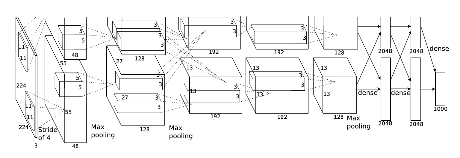
An illustration of the architecture of our CNN, explicitly showing the delineation of responsibilities between the two GPUs. One GPU runs the layer-parts at the top of the figure while the other runs the layer-parts at the bottom. The GPUs communicate only at certain layers. The network’s input is 150,528-dimensional, and the number of neurons in the network’s remaining layers is given by 253,440–186,624–64,896–64,896–43,264– 4096–4096–1000.
As we can see here, AlexNet features 8 layers, the first 5 being convolutional and the last three being fully-connected (FC) layers. The output layer is processed by a softmax function, which produces a distribution of probabilities across 1000 labels, classifying the input images.Normalization and max-pooling layers are implemented at several locations, and the choice of activation function is ReLU throughout the network.
Dropout is also used to reduce overfitting. As described in the original papaer, “We use dropout in the first two fully-connected layers of Figure 2. Without dropout, our network exhibits substantial overfitting. Dropout roughly doubles the number of iterations required to converge.”.
Additional Notes
Although 8 layers does not make a very deep neural network by today’s standard, the computational power required was already very high compared to earlier networks. Take LeNet by LeCun from 1998 as an example (which has often been credited as the first functional CNN) - it has 2 convolutional layers and 2 FC layers. In fact, as Alex once said in a conference talk, the idea for AlexNet was basically an intention to re-implement the original LeNet architecture, but make use of multiple GPUs for faster computation, and thus enabling the CNN to work with deeper layers, which resulted in AlexNet. As the quote and the diagram illustrates, there are two GPUs working parallelly on the network, communicating at certain layers. For our purpose, we will not bother with the intricacies of such, but emphasize the structure of the network itself. The original training process also used data augmentation (reflections, random patch extractions, slight rotations, etc.) to reduce overfitting, and we will only briefly touch upon this when we implement the MNIST example at the end.
Summary
We summarize the approximate structure in the table below.
| Layer | Size | Kernel | Channel | Stride | Activation | |
|---|---|---|---|---|---|---|
| Input | image | 224*224*3 | 3 | |||
| 1 | Convolution | 55*55*96 | 11*11 | 96 | 4 | ReLU |
| Max Pooling | 27*27*96 | 3*3 | 96 | 2 | ReLU | |
| 2 | Convolution | 27*27*256 | 5*5 | 256 | 1 | ReLU |
| Max Pooling | 13*13*256 | 3*3 | 256 | 2 | ReLU | |
| 3 | Convolution | 13*13*384 | 3*3 | 384 | 1 | ReLU |
| 4 | Convolution | 13*13*384 | 3*3 | 384 | 1 | ReLU |
| 5 | Convolution | 13*13*256 | 3*3 | 256 | 1 | ReLU |
| Max Pooling | 4*4*256 | 3*3 | 256 | 2 | ReLU | |
| 6 | Fully Connected | 4096 | ReLU | |||
| Dropout | ||||||
| 7 | Fully Connected | 4096 | ReLU | |||
| Dropout | ||||||
| 8 / Output | Fully Connected | 1000 | Softmax | |||
Using AlexNet in Keras
Now, let’s get started exploring AlexNet in Keras. First you will need to setup Keras - the exact process will depdend on your platform and environment, but there are many resources out there you could use as reference. Assuming we are ready to go, I’ll get started with the codes.
Imports
First we import the modules that we would use
import keras
from keras.models import Sequential
from keras.layers import Dense, Activation, Dropout, Flatten, Conv2D, MaxPooling2D
from keras.layers.normalization import BatchNormalization
import numpy as np
Building the Network
Next we build up the network using the summary table above.
# Instantiate a Sequential model
model = Sequential()

# 1st Convolutional Layer
model.add(Conv2D(filters=96, input_shape=(224, 224, 3), kernel_size=(11, 11), strides=(4, 4), padding='valid'))
model.add(Activation('relu'))
# Max Pooling
model.add(MaxPooling2D(pool_size=(3, 3), strides=(2, 2), padding='valid'))

# 2nd Convolutional Layer
model.add(Conv2D(filters=256, kernel_size=(5, 5), strides=(1, 1), padding='valid'))
model.add(Activation('relu'))
# Max Pooling
model.add(MaxPooling2D(pool_size=(3, 3), strides=(2, 2), padding='valid'))

# 3rd Convolutional Layer
model.add(Conv2D(filters=384, kernel_size=(3, 3), strides=(1, 1), padding='valid'))
model.add(Activation('relu'))

# 4th Convolutional Layer
model.add(Conv2D(filters=384, kernel_size=(3, 3), strides=(1, 1), padding='valid'))
model.add(Activation('relu'))

# 5th Convolutional Layer
model.add(Conv2D(filters=256, kernel_size=(3, 3), strides=(1, 1), padding='valid'))
model.add(Activation('relu'))
# Max Pooling
model.add(MaxPooling2D(pool_size=(3, 3), strides=(2, 2), padding='valid'))

# Fully Connected layer
model.add(Flatten())
# 1st Fully Connected Layer
model.add(Dense(4096, input_shape=(224*224*3,)))
model.add(Activation('relu'))
# Add Dropout to prevent overfitting
model.add(Dropout(0.5))

# 2nd Fully Connected Layer
model.add(Dense(4096))
model.add(Activation('relu'))
# Add Dropout
model.add(Dropout(0.5))

# Output Layer
model.add(Dense(1000))
model.add(Activation('softmax'))

model.summary()

# Compile the model
model.compile(loss=keras.losses.categorical_crossentropy, optimizer='adam', metrics=['accuracy'])
The compiled model should return a summary of the architecture:
_________________________________________________________________
Layer (type)                 Output Shape              Param #
=================================================================
conv2d_6 (Conv2D)            (None, 54, 54, 96)        34944
_________________________________________________________________
activation_6 (Activation)    (None, 54, 54, 96)        0
_________________________________________________________________
max_pooling2d_4 (MaxPooling2 (None, 26, 26, 96)        0
_________________________________________________________________
conv2d_7 (Conv2D)            (None, 22, 22, 256)       614656
_________________________________________________________________
activation_7 (Activation)    (None, 22, 22, 256)       0
_________________________________________________________________
max_pooling2d_5 (MaxPooling2 (None, 10, 10, 256)       0
_________________________________________________________________
conv2d_8 (Conv2D)            (None, 8, 8, 384)         885120
_________________________________________________________________
activation_8 (Activation)    (None, 8, 8, 384)         0
_________________________________________________________________
conv2d_9 (Conv2D)            (None, 6, 6, 384)         1327488
_________________________________________________________________
activation_9 (Activation)    (None, 6, 6, 384)         0
_________________________________________________________________
conv2d_10 (Conv2D)           (None, 4, 4, 256)         884992
_________________________________________________________________
activation_10 (Activation)   (None, 4, 4, 256)         0
_________________________________________________________________
max_pooling2d_6 (MaxPooling2 (None, 1, 1, 256)         0
_________________________________________________________________
flatten_1 (Flatten)          (None, 256)               0
_________________________________________________________________
dense_1 (Dense)              (None, 4096)              1052672
_________________________________________________________________
activation_11 (Activation)   (None, 4096)              0
_________________________________________________________________
dropout_1 (Dropout)          (None, 4096)              0
_________________________________________________________________
dense_2 (Dense)              (None, 4096)              16781312
_________________________________________________________________
activation_12 (Activation)   (None, 4096)              0
_________________________________________________________________
dropout_2 (Dropout)          (None, 4096)              0
_________________________________________________________________
dense_3 (Dense)              (None, 1000)              4097000
_________________________________________________________________
activation_13 (Activation)   (None, 1000)              0
=================================================================
Total params: 25,678,184
Trainable params: 25,678,184
Non-trainable params: 0
_________________________________________________________________
It’s actually that simple - we now have an (approximate) AlexNet compiled and ready to train. However, to make things a bit easier on machines not that powerful, we will implement a dumbed-down version of AlexNet, on a classic dataset called “MNIST”, which consists of hand-written digits, and the task would be to recognize which digit each image corresponds to. Let’s get started.
Example: Keras + MNIST
As usual, let’s build a simple neural network, reminiscent of the structure of AlexNet. Then we will import the dataset provided by Keras, train and fit the model, and discuss some of our findings. The codes below will be carefully commented but should there be anything unclear, please leave a comment below and I will be glad to help explain what’s going on!
# Some modules / packages we will use to help with the process
# If you encounter errors such as Module not found, please make sure to
# install the packages below first
import numpy as np
import pandas as pd
import matplotlib.pyplot as plt
%matplotlib inline

# load MNIST dataset
from keras.datasets import mnist

from keras.models import Sequential
from keras.layers import Dense, Dropout, Activation, Flatten
from keras.optimizers import Adam
from keras.layers.normalization import BatchNormalization
from keras.utils import np_utils
from keras.layers import Conv2D, MaxPooling2D, ZeroPadding2D, GlobalAveragePooling2D
# from keras.layers.advanced_activations import LeakyReLU
from keras.preprocessing.image import ImageDataGenerator

#################################################
# Step 1:
# Load the image data
(X_train, y_train), (X_test, y_test) = mnist.load_data()

"""
X_train:

We can play around with the loaded images a bit
We will see that X_train is (60000, 28, 28), so that we have
60000 training images, each with a 28*28 resolution

y_train:
This is an array of labels. For example - y_train[:20] is
array([5, 0, 4, 1, 9, 2, 1, 3, 1, 4, 3, 5, 3, 6, 1, 7, 2, 8, 6, 9],
      dtype=uint8)

Each label shows what digit the corresponding image in X_train is.
"""


#################################################
# Step 2:
# Pre-processing the data into desired format

"""
I am using Keras with TensorFlow backend, and that requires
the input to be in a specific format: (batch, height, width, channels)

if you are using Theano backend, you might need to preprocess the
input into a different format, possibly (batch, channels, height, width).

"""
# reshape into (batch, height, width, channels)
# we have 60000 training images and 10000 testing images
X_train = X_train.reshape(60000, 28, 28, 1)
X_test = X_test.reshape(10000, 28, 28, 1)

# Normalize to float between 0 and 1
# Original pixel values are between 0 and 255
X_train = X_train.astype('float32')
X_test = X_test.astype('float32')
X_train = X_train / 255
X_test = X_test / 255

"""
For y_ label data, we want to convert them into categorical / one-hot variables.
In our case, we have 10 categories, so for example, for our first label in
y_train, the value is 5, then we want to convert it into
[0, 0, 0, 0, 0, 1, 0, 0, 0, 0], with the index of 1 indicating the value of y_train[0]
"""

# keras.utils.np_utils conveniently has this built in
classes = 10
y_train = np_utils.to_categorical(y_train, classes)
y_test = np_utils.to_categorical(y_test, classes)


#################################################
# Step 3:
# Build our Neural Network

# As earlier, but with much lower dimensions and fewer layers
# (since our input is 28*28 images anyway)
# Instantiate a Sequential model
model = Sequential()

# 1st Convolutional Layer
model.add(Conv2D(filters=32, input_shape=(28, 28, 1), kernel_size=(3, 3), strides=(1, 1), padding='valid'))
model.add(Activation('relu'))
# Max Pooling
model.add(MaxPooling2D(pool_size=(3, 3), strides=(1, 1), padding='valid'))

# 2nd Convolutional Layer
model.add(Conv2D(filters=32, kernel_size=(3, 3), strides=(1, 1), padding='valid'))
model.add(Activation('relu'))
# Max Pooling
model.add(MaxPooling2D(pool_size=(3, 3), strides=(1, 1), padding='valid'))

# 3rd Convolutional Layer
model.add(Conv2D(filters=64, kernel_size=(3, 3), strides=(1, 1), padding='valid'))
model.add(Activation('relu'))

# 4th Convolutional Layer
model.add(Conv2D(filters=64, kernel_size=(3, 3), strides=(1, 1), padding='valid'))
model.add(Activation('relu'))

# Max Pooling
model.add(MaxPooling2D(pool_size=(3, 3), strides=(2, 2), padding='valid'))

# Fully Connected layer
model.add(Flatten())
# 1st Fully Connected Layer
model.add(Dense(512))
model.add(Activation('relu'))
# Add Dropout to prevent overfitting
model.add(Dropout(0.3))

# Output Layer
# important to have dense 10, since we have 10 classes
model.add(Dense(10))
model.add(Activation('softmax'))

model.summary()

# Compile the model
model.compile(loss=keras.losses.categorical_crossentropy, optimizer='adam', metrics=['accuracy'])


#################################################
# Step 4:
# Prepare for training

# We use ImageDataGenerator to augment our input data
# which among other benefits, can help reduce over-fitting
gen = ImageDataGenerator(
            rotation_range=8,
            width_shift_range=0.08,
            shear_range=0.3,
            height_shift_range=0.08,
            zoom_range=0.08
            )
test_gen = ImageDataGenerator()

# hyoer-parameters
# We train in batches to speed up the process
# (and so that our memory can handle the data)
BATCH_SIZE = 64
# How many rounds of training? Let's start from a smaller number
EPOCHS = 5

# Generator to "flow" in the input images and labels into our model
# Takes batch_size as a parameter
train_generator = gen.flow(X_train, y_train, batch_size=BATCH_SIZE)
test_generator = test_gen.flow(X_test, y_test, batch_size=BATCH_SIZE)

#################################################
# Step 5:
# Do the training!
model.fit_generator(
        train_generator,
        steps_per_epoch=60000//BATCH_SIZE,
        epochs=EPOCHS,
        validation_data=test_generator,
        validation_steps=10000//BATCH_SIZE
        )

"""
This should run for a little while, printing some progress in the process:

Epoch 1/5
937/937 [==============================] - 173s 184ms/step - loss: 0.2400 - acc: 0.9240 - val_loss: 0.0492 - val_acc: 0.9848
Epoch 2/5
937/937 [==============================] - 171s 182ms/step - loss: 0.0841 - acc: 0.9742 - val_loss: 0.0304 - val_acc: 0.9899
Epoch 3/5
937/937 [==============================] - 170s 181ms/step - loss: 0.0638 - acc: 0.9803 - val_loss: 0.0358 - val_acc: 0.9902
Epoch 4/5
937/937 [==============================] - 163s 173ms/step - loss: 0.0532 - acc: 0.9836 - val_loss: 0.0197 - val_acc: 0.9936
Epoch 5/5
937/937 [==============================] - 167s 179ms/step - loss: 0.0495 - acc: 0.9849 - val_loss: 0.0227 - val_acc: 0.9934

We see at 5 epochs, we are achieving impressive results with a validation accuracy at 99.34%.
"""

#################################################
# Step 6:
# Do some predictions

# Ideally we would want to use some new iamges to play with predictions
# but lets just grab some from the test set

# Take first image in testing dataset
to_predict = X_test[0]
# reshape from (28, 28, 1) --> (1, 28, 28, 1)
to_predict = np.expand_dims(to_predict, axis=0)

# make prediction: this gives probability distribution
# over all classes
model.predict(to_predict)

# This returns the class with the highest probability
model.predict_classes(to_predict)
# --> array([7], dtype=int64)

# Let's compare with actual label:
y_test[0]
# array([0., 0., 0., 0., 0., 0., 0., 1., 0., 0.], dtype=float32)

# Indeed, the first image in test set has an actual label of index 7,
# as our model has correctly predicted.

#################################################
# Step 7:
# Save your model

"""
Although this particular model was pretty fast to train,
sometimes our model would actually take a long time to train,
and it would be quite disappointing if we need to retrain these models
everytime we use them, yes?

Thankfully, we can easily save and reload them whenever we need.
"""
from keras.models import load_model

model.save('my_mnist_model.h5')

# When we need to load it back
# we can just run
model = load_model('my_mnist_model.h5')
# and get the same model object as earlier.
Bonus Visualize
Curious what the image we had made prediction on looks like? Here you go:

Conclusion
In this post, we have explored and implemented AlexNet, and played around with an actual example of digit recognition using a simplified CNN, all done using Keras. We have witnessed nowadays, how easy it is to play around and explore neural networks with such high-level apis such as Keras, casually achieving very high accuracy rate with just a few lines of codes. In the real world, of course, with much more complex challenges, things are not going to be as smooth as we see here, but the basic strategy still holds. In the next post, let us explore some more recent landmark networks, to study and discuss how they work and why they work well.

Leave a comment