Neural Networks - 5. Convolutional Neural Networks: Case Studies (1)

Links to Other Parts of Series

• Neural Network Series

Overview

In this post in our Neural Network series, we will look into a few landmark Convolutional Neural Networks. We will look at the structure of each network, try to understand the idea behind the implemented structures, and hopefully be able to take away some helpful points we could apply to our own network designs in the future. To give a summary, we will look at the following networks: VGG (2014), GoogLeNet/Inception (2014), ResNet (2015), WideResNet (2016), DenseNet (2017), Squeeze-and-Excitation Networks (2017), and EfficientNet (2019). We will cover the first 4 in this week’s post, and the latter 3 in our next post.

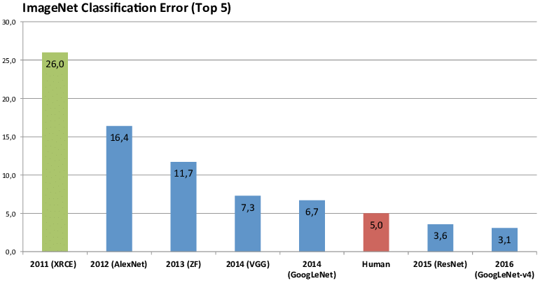
The graph below shows the achievements of some of the networks mentioned above - as we can see, many of them are among the best performing networks of their time, by the metrics of their error rate on ImageNet Large Scale Visual Recognition Challenge (ILSVRC). We have covered AlexNet (2012) extensively in our previous post, so this time around, we will start with its successor, the VGG network.

(source)

Networks

VGG

VGG stands for Visual Geometry Group based in University of Oxford. They showed in their VGG networks that without departing from the classical ConvNet architecture (e.g. LeCun 1989), their model was able to achieve significantly better results by increasing the depth. They configured several variations of the networks, but the two most famous variations would be VGG 16 and VGG 19 (partly due to them making their trained weights publicly available), which, unsurprisingly, has 16 and 19 layers, respectively. Although not very deep by today’s standard, they were indeed among the deepest nets at that time.

Structure

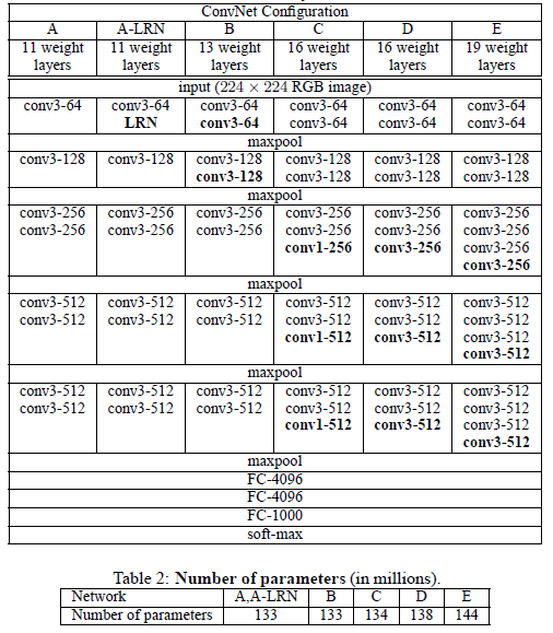
(source: [1] )

As we can see, the networks in general consists of 3-by-3 convolutional layers, with sporadic max-poolings. ReLU was chosen as the activation functions, and a softmax is applied to the output layer, to predict the distribution of probabilities across the 1000 class of objects.

Points of Interest

1. In configuration C above, conv1-X layers has been introduced. This was an attempt to increase non-linearity of the decision function (through the ReLU activations) without affecting the receptive fields of the convolutional layers. Although VGG’s implementation of 1x1 conv. layers are of the same channel-dimensions as previous layers, such “Network in Network” architecture has been used in other networks for other purposes, such as reducing the dimensionalities (through fewer channels).
2. Since the general structure is made up of 3x3 layers, we would like to compare two things: A. multiple 3x3 layers stacked in depth, and B. a single layer of larger dimension.
   • Case A: It is not hard to see that two 3x3 layers has the same amount of effective receptive fields as a single 5x5 layer (since as the conv. layers scans through the first layer, it effectively expands the layer by 1 pixel on each side). Similarly, three 3x3 layers has effectively the same fields as a single 7x7 layer. With three 3x3 layers, we would have 27 parameters to train for each channel.
   • Case B: For our 7x7 layer, we would need 49 parameters per channel.
   • As the authors argue, this three 3x3 layers implementation can be viewed as some sort of regularisation requirement on the 7x7 layer, since it imposes this decomposition through the multiple 3x3 layers.
3. As a result of the point above, although the network is much deeper than earlier versions, the total number of parameters to train is not greter than other shallower networks with conv. layers of higher dimensions.
4. In their training and evaluation phase, they have experimented with scale jittering at training time, and achieved better results with such variations in training data. This confirms that “training set augmentation by scale jittering is indeed helpful for capturing multi-scale image statistics” [1].
5. ConvNet Fusion: by using an ensemble of multiple models (making predictions based on the average predicted probabilties across variations of the network), they were able to achieve higher accuracy rate than any single model’s individual predictions.
6. Note that although the authors demonstrated that “representation depth is beneficial for the classification accuracy, [……] results yet again confirm the improtance of depth in visual representations”, it is actually not entirely clear whether it is the depth alone led to the improved performance. As we will see later, there are others who will explore other channels of improvement, and would argue that despite the trend of building deeper networks, many other factors could contribute to the performance.

GoogLeNet/Inception

GoogLeNet, code named “Inception”, implements a Network-in-Network architecture that sets out to mimic the sparse structure of our biological system, which correspondes better to neuroscience models of primate visions. The building block is a so called “Inception module”, which we will introduce below.

Structure

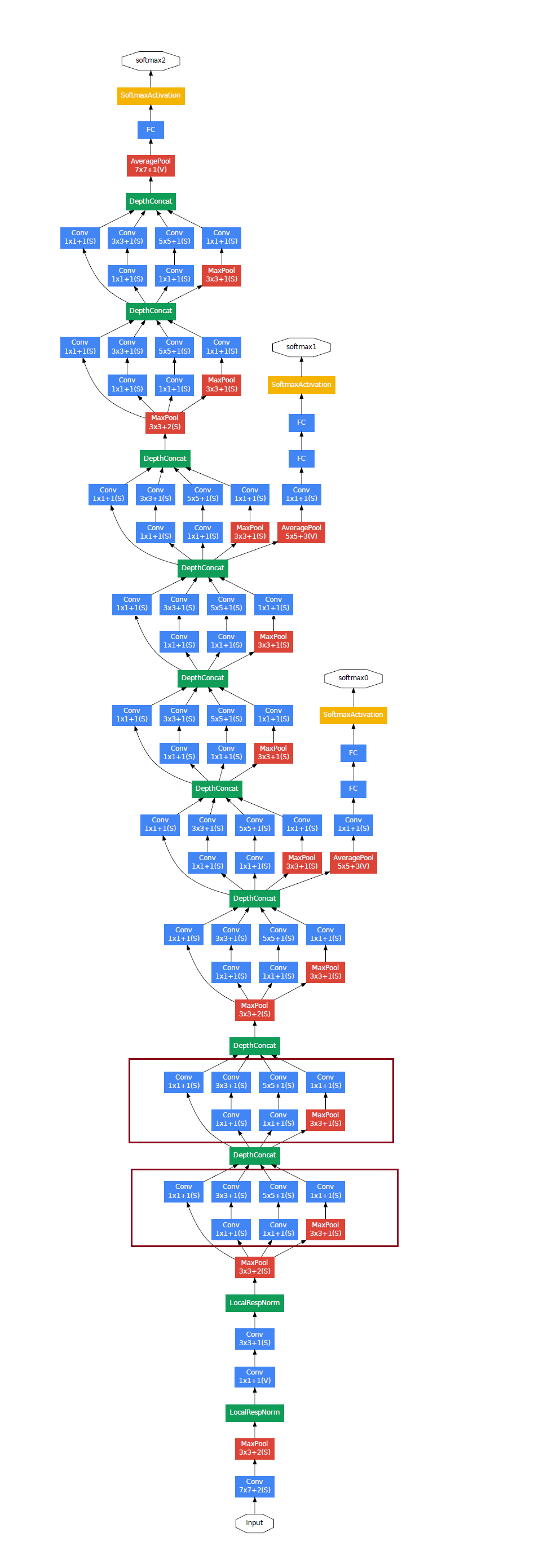
(source: [2])

As we can see, this 22-layer network structure mostly consists of this repeating components shown below (and boxed in red above):

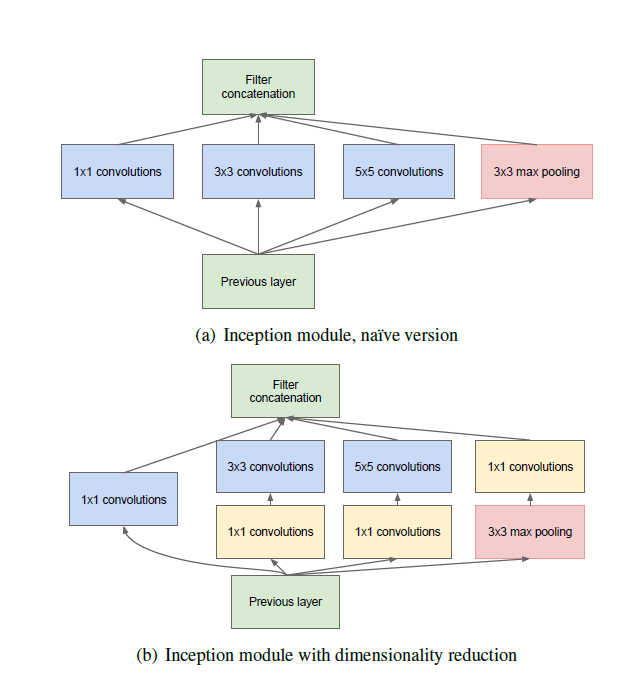
(source: [2])

This inception module is made up of a collection of 1x1, 3x3, 5x5 and a max-pooling layer. Before the inputs are passed into the 3x3 and 5x5 conv layers, and after the max-pooling layer, a 1x1 convolution was applied. Keeping these in mind, let’s talk about some interesting points presented by this network as well as the accompanying paper [2].

Points of Interest

1. The accompanying paper, “Going Deeper with Convolutions”, implied 2 different meanings of “deeper”: on one hand there is the “inception module” that increased the organizational depth of the model, while on the other, it quite literally increased the depth of the network.
2. As with VGG, this model was also developed with efficiency in mind - depth and width are increased, but computational budget was kept constant.
3. The construction of the inception module is in part inspired by neuroscience and in particular, multi-scale processing, where each conv layer of a specific size is intended to capture different types of features.
4. 1x1 convolutional layers are heavily deployed - as we have seen in VGG, these layers are able to provide additional non-linearity for the models. However, in this particular network, the 1x1 conv layers are mostly used for dimension reduction, in an effort to remove computational bottlenecks. In essence, the 1x1 conv layers condensed multiple channels from the previous layers into fewer channels, and hence reducing the depth of the inception layer. This technique allowed the computational burden of the Inception network to be kept at a reasonable level. Intuitively, as the paper described, “the design follows the practical intuition that visual information should be processed at various scales and then aggregated so that the next stage can abstract features from the different scales simultaneously.”
5. If we take a closer look at the overall structure above, we will notice 2 auxiliary softmax / classification branches. These were implemented in an attempt to mitigate the vanishing gradient issue that is common among deep neural networks. The idea is that, since shallower networks are able to achieve decent classification results, if we add some auxiliary classification branches at some intermediate layers, they should produce somewhat meaning results, which we could use to help with the Cost function computation, and therefore help with gradient descent and backpropagation process.However, they have discovered that the effect of these auxiliary networks and branches is relatively minor at best.
6. They also incorporated ensemble predictions of several versions of the model, differing only in sampling methodologies and input image orders.

ResNet

ResNet here stands for Residual Neural Network. The distinctive feature it uses in its network are “shortcut connections”, as we will see below, where an addtional identity mapping is attached to the building blocks, making the resulting block essentially training to learn the residual. It was a highly successful model, in that it has won 1st place in the ILSVRC 2015 classification competition with top-5 error rate of 3.57%, and also performing very well on other datasets / tasks.

Structure

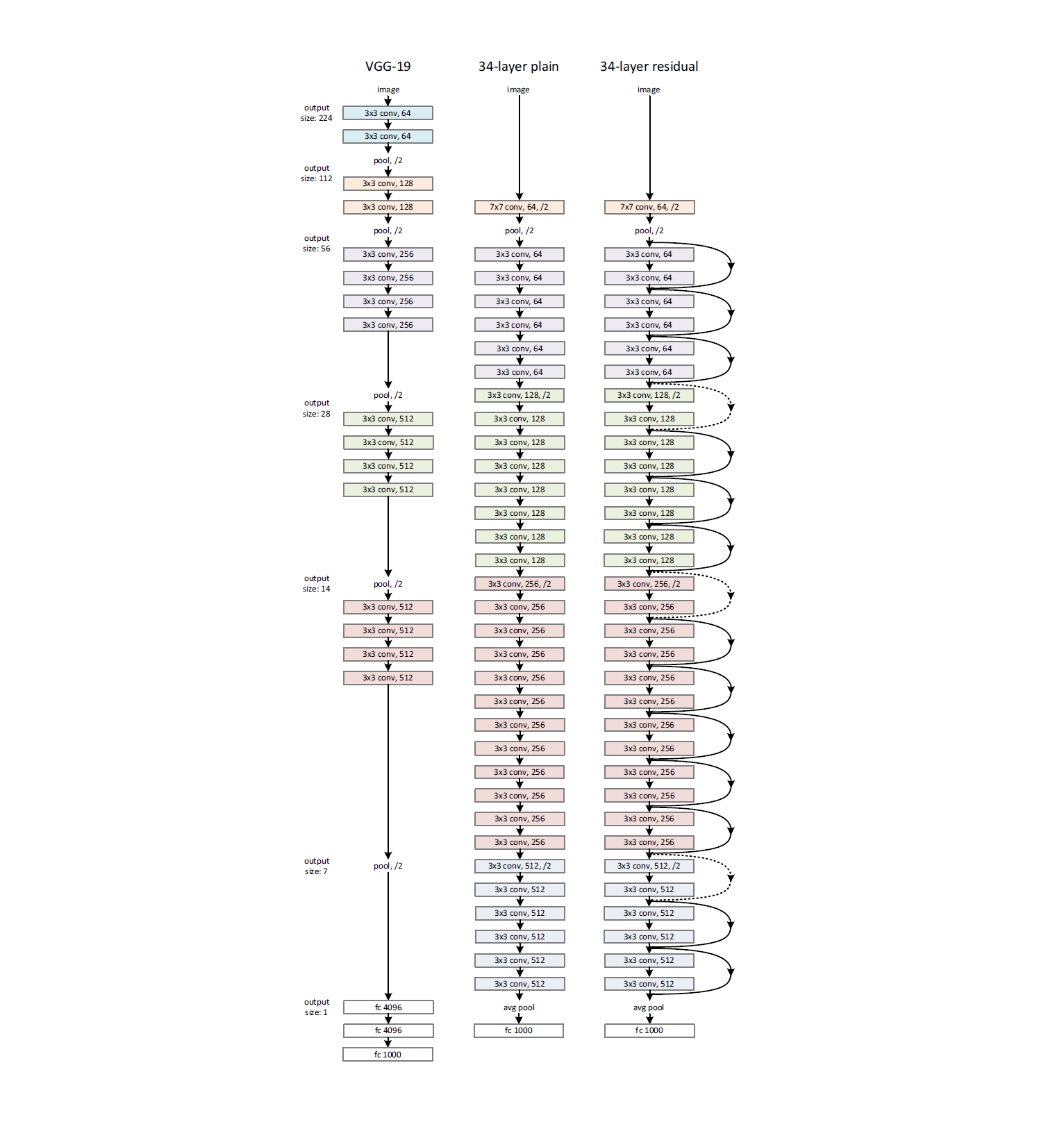
(source: [3])

The figure above shows the 34-layer version of the ResNet, along with its plain net coparision (no shortcut connections), and a VGG-19. Notice that the common ResNet we are refering to is usually the 152-layer version, but this 34-layer illustration suffices to help us understand the idea. Take another look at this architecture, and then let’s talk about some points of interest.

Points of Interest

1. It is generally understood that deeper networks can better integrate low/mid and high-level features, which should result in better network performance in terms of classifying or detecting objects. However, a notorious issue with deep neural networks is vanishing gradient.
2. Vanishing gradient has been partially addressed by normalized initializations paired with intermediate normalization layers.
3. However, another issue deep neural networks faces is a degradation problem, i.e. accuracy gets saturated and then degrades rapidly. In addition, this does not seem to be caused by overfitting, as even training error is higher with deeper networks after a certain point. The authors of ResNet compared their 18-layer and 34-layer plain nets, and confirmed this point. The authors have shown in their results that after implementing these measures, the particular optimization challenge they can still observe is unlikely to be caused by vanishing gradients.
4. This indicates that deeper networks might simply be too hard to optimize. In theory, by construction, a deeper network should be able to perform at least as well as a shallower network, since all it needs to do is to set the remaining layers to mimic identity mappings. However, the observed degradation problem “suggests that the solvers might have difficulties in approximating identity mappings by multiple nonlinear layers”.
5. ResNet mainly aims to address this issue. With an identity “shortcut connection”, the network can learn identity mapping simply by driving the residual to 0, which is much easier to do than the original challenge. In particular, if we denote H(x) to be the underlying non-linear function, and x be the identity mapping, then our model should now try to fit the stacked non-leanr layers to F(x):= H(x) - x, the residual of the underlying non-linearity, after subtracting the identity.
6. Notice that these shortcut connections / identify mappings, do not increase parameters nor computational complexities (aside from some trivial additions). For comparison, their 152-layer network still has a lower complexity when compared to VGG-16 / VGG-19.
7. The authors of ResNet has shown that based on their results, after the addition of these shortcut connections, the degradation issue is no longer observed (deeper network has at least lower training errors). This (along with ) allowed them to implement deeper networks, and “enjoy accuracy gains from greatly increased depth, producing results substantially better than previous networks”.

WideResNet (WRNs)

As the state of the art results on various challenges are being achieved by deeper and deeper networks, people start noticing that the improvements in accuracy with regards to the number of layers is diminishing quickly, and as networks get deeper and deeper, they become slower and slower to train. The authors of this paper ([4]) proposes to explore the width (number of channels/filters) along with the depth, and demonstrated that modifying the calssic ResNet but with fewer layers and more channels within each residual block, their 16-layer-deep WRN “outperforms in accuracy and efficiency all previous deep residual networks”.

Structure

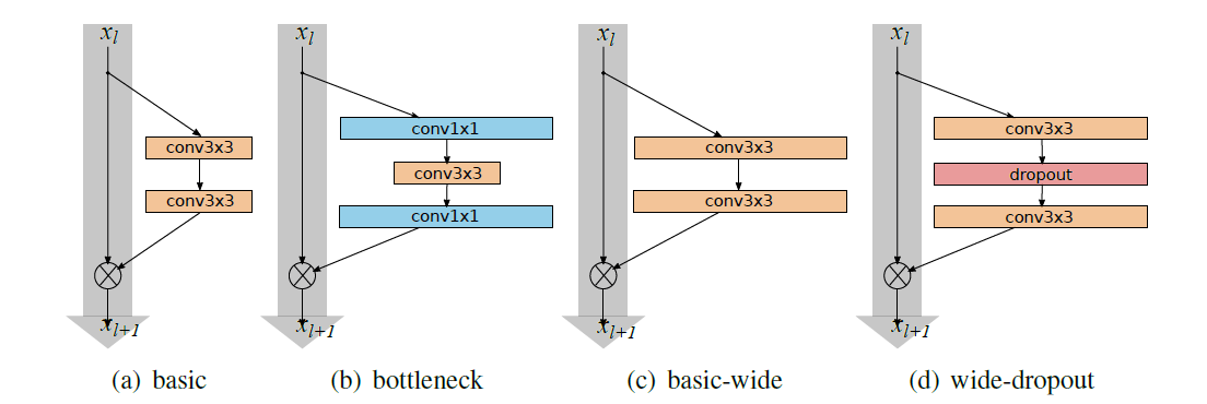
(source: [4])

The basic structure is of the same spirit as to the ResNet architecture, but with one twist where within each residual block, they have increased the number of filters by a factor of k, along with an added dropout layer in between the conv layers (structure d).

Points of Interest

1. ResNet was made very “thin” in an attempt to keep the total number of parameters at check, while increasing the depth of the network. However, the authors of this paper argues that it might just be the residual blocks working wonders, while the depth is not that crucial. The idea of wider network is nothing new - most networks before ResNet were fairly wide - so the idea is that perhaps depth is only supplementary in this context, and implementing wider residual blocks could lead to overall improvements.
2. In fact, they attempt to show that “the widening of ResNet blocks (if done properly) provides a much more effective way of improving performance of residual neural networks compared to increasing their depth.”
3. Their 16-layer WRN has the same accuracy as the 1000-layer thin network, with comparable amount of parameters but much faster to train (since GPUs can take advantages of width better than depth through parallel computing).
4. They have experimented with different combinations of depth x width, and while both depth and width helps, after a certain point, the parameters become too much and stronger regularization is needed. In this regard, wide networks can successfully learn significantly more parameters than thin ones.
5. The state of the art results were achieved through a WRN approximately 28 layers deep and 10-12 k factors wide (10-12 times the number of filters compared to ResNet).

Conclusion

In this post we have reviewed a couple of landmark papers / neural networks, getting a sense of how things have been developing and the trend in CNN research. In the next post, we will continue on this journey to study a couple of more recent advances in the field. Stay tuned!

Resources

References:

[1] Simonyan, Karen, and Andrew Zisserman. “Very deep convolutional networks for large-scale image recognition.” arXiv preprint arXiv:1409.1556 (2014).

[2] Szegedy, Christian, et al. “Going deeper with convolutions.” Proceedings of the IEEE conference on computer vision and pattern recognition. 2015.

[3] He, Kaiming, et al. “Deep residual learning for image recognition.” Proceedings of the IEEE conference on computer vision and pattern recognition. 2016.

[4] Zagoruyko, Sergey, and Nikos Komodakis. “Wide residual networks.” arXiv preprint arXiv:1605.07146 (2016).