Neural Networks - 1. Overview

Links to Other Parts of Series

• Neural Network Series

Overview

In this series of blog posts we will explore one of the most important building blocks in Deep Learning: Neural Networks. We will explore various Deep Neural Networks (DNN), including Convolutional Neural Networks (CNN) and Recurrent Neural Networks (RNN). We will explore the theories behind them, code implementations, as well as real-world applications. In this first part, we will give an overview of the landscape.

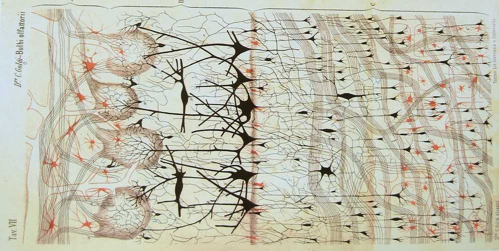
Deep learning is part of Machine Learning that is based on artificial neural networks. The structure of such networks is often reminiscent of neural networks of human brains, as shown in the drawing above: nodes are connected to numerous other nodes, processing signals from one end to the other, selectively activating nodes in between. “Deep Learning”, “Deep Neural Networks” (DNN), “Convolutional Neural Networks” (CNN)… Don’t be intimidated, or get over excited by these big words - Deep Learning folks love to lure people in using cool terminologies, but at the end of the day, once you are lured in, you will discover that, for better or worse, it’s all linear algebra, calculus, and probability in disguise. Before all that good stuff, let’s first get some intuitions.

The Different Types of Neural Networks

There are many types of neural networks, but at a high level, most common architectures you will be able to find when exploring on your own will probably fall into one of the following categories:

• Convolutional Neural Networks
• Recurrent Neural Networks

Convolutional Neural Networks

Convolutional Neural Networks (CNNs) are a type of network that are commonly used for feature extraction algorithims, such as image classifications, image recognitions. As the diagram above indicates, CNNs operates in a series of layers, where usually the dimension of the problem is gradually reduced, and the feature being extracted is more and more high level. This can be visualized below:

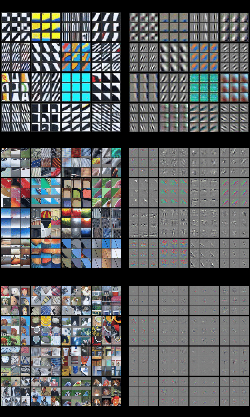
Images on the left are original images being processed, while the corresponding results on the right are the features that are most “activated” on that specific layer. Starting from the top to bottom panels, we can see that as we go deeper into the layers, we gradually shift from blurry lines, curvy edges, to more human-recognizable features. For image classification problems, we can kind of see how as the layers get deeper, the algorithm may be able to determine whether the input was a car, a bicycle, a flower, or a dog.

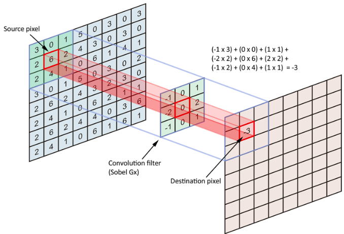
So what is each layer? As we’ve mentioned earlier, it’s all math. Using an image as an example, we can represent it as arrays of numbers. Then, each layer in a network is essentially performing some sort of operation on these matrices, which we sometimes call “filters”. The example below (source) shows a Sobel filter, where a 3-by-3 sub-matrix is processed into a single number. The resulting layer will usually be processed by going through an activation function, which introduces non-linearities into our model. Non-linearity creates possibilities, and enables our model to capture more complex features. The result will then be passed through later layers, such as pooling, normalization, another filter, or any other kind of layers.

When we talk about training a network, it is usually referring to the process of fine-tuning the weights on each node / neuron. Think about the image classification example again, where we gave the network an image of a car as the input. The network reads in the car as a multi-dimensional array, the values in the arrays gets passed through the layers of the network, but the particular value that is outputed by the network depends on the parameters of each layers. In order to tune the parameters, we need to define a goal, so that we can evaluate how well the current parameters are doing. This is often done by specifying a Cost Function, which intuitively represents the distance between the ideal output, and the particular output generated by our network. We then use a technique called Back Propagation to find improvements to the current network parameters, until we are happy with the trained parameters, or the improvements are becoming minimal after each run. We will talk about these in more details in our blog post dedicated to CNNs.

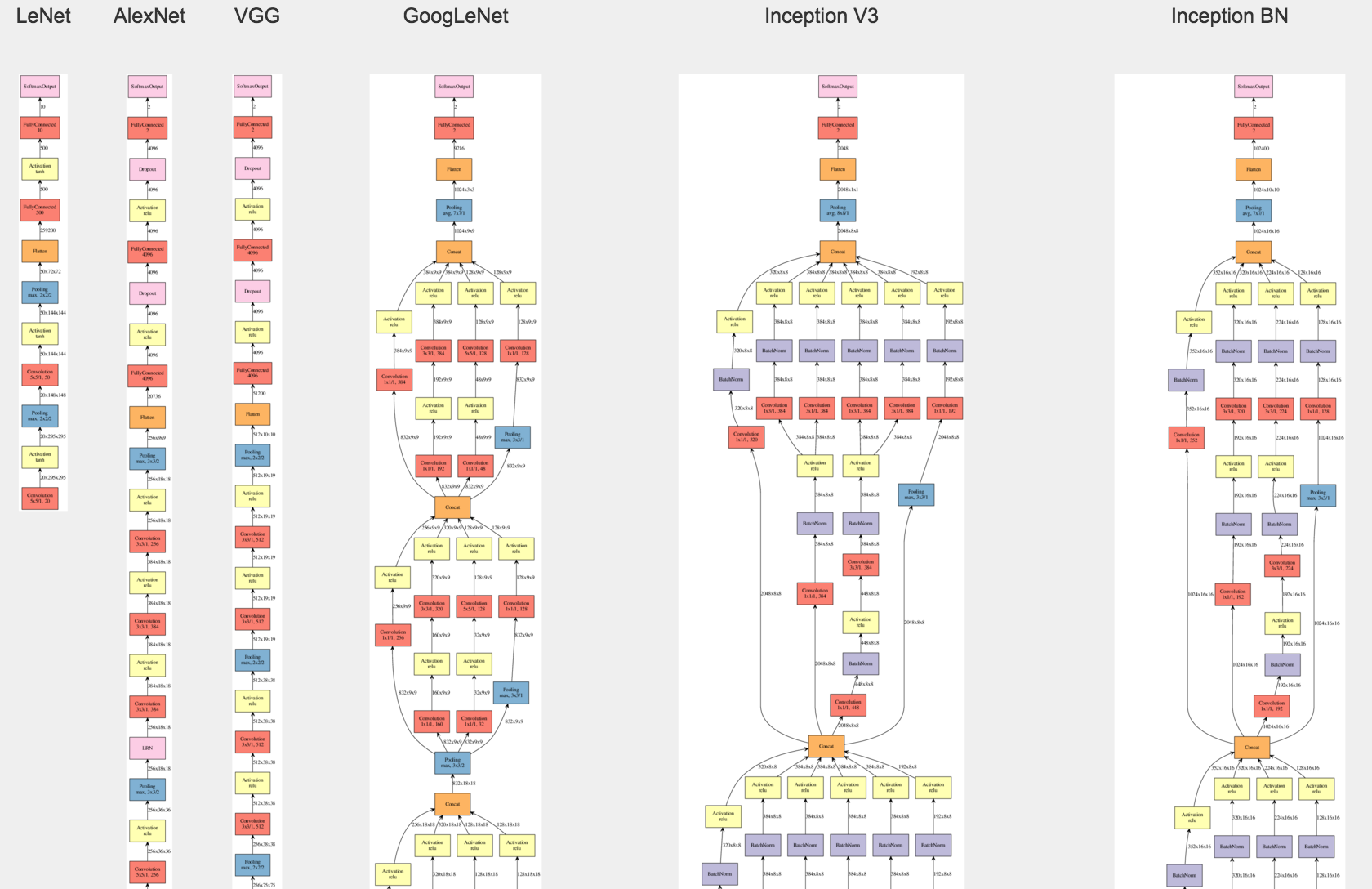
Various implementation of CNNs usually differ in how each layer is structured, how information from one layer is passed to another layer. I found a very helpful visualization here, where the author visualizes several important CNNs through 2015. Looking at the thumbnail, Without even checking out the details, it’s easy to tell that the structure of CNNs has become more and more involved, and more often than not, growing deeper as well.

Applications of CNNs are everywhere. Autonomous cars, objects detections, facial recoginition, medical applications (image diagnosis), and so on. We will examine the details of this network in a separate post, but the message to take away is, CNN is really good at recognizing features from an input image, and each layer is usually “activated” by a particular type of feature.

Recurrent Neural Networks

The main distinctive feature of RNNs, compared to CNNs, is that CNNs are feedforward neural networks, in the sense that the input is processed in a one-way fashion, where it goes through the layers of the network only once. They take an input image, and returns an output, and that’s it. On the other hand, RNNs are adept at handling sequential data, such as words in a sentence; nodes and neurons in RNN can process signals not only from the current input, but also inputs from other temporal stages, which makes it suitable for applications where capturing long-term dependency is required within the data itself. Again, let us start with an example.

A particular class of architecture in RNNs is LSTM, which stands for Long Short Term Memory. Suppose a user is typing out a document, and we want to help make suggestions as to what the next word might be. To train our LSTM model, we feed the model some texts the users have already typed out, for exmaple:

Deep learning is part of Machine Learning that is based on artificial neural networks. The structure of such networks is often reminiscent of neural networks of human brains, as shown in the drawing above: nodes are connected to numerous other nodes, processing signals from one end to the other, selectively activating nodes in between. “Deep Learning”, “Deep Neural Networks” (DNN), “Convolutional Neural Networks” (CNN)… Don’t be intimidated, or get over excited by these big words - Deep Learning folks love to lure people in using cool terminologies, but at the end of the day, once you are lured in, you will discover that, for better or worse, it’s all linear algebra, calculus, and probability in disguise. Before all that good stuff, let’s first get some intuitions.

And the user continues to type, for example, “the next type of neural “, and at this particular moment, we want our LSTM model to predict the next word.

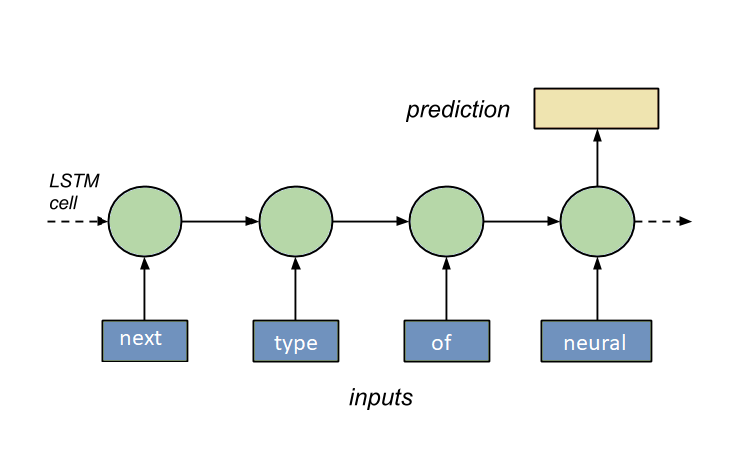
If our model is well trained, it shouldn’t be too difficult to figure that, after “neural”, more often than not comes the word “network”. In real applications, however, the case is often not too clear even to human brains, and so to successfully train an LSTM model to do reasonably well is no small feat.

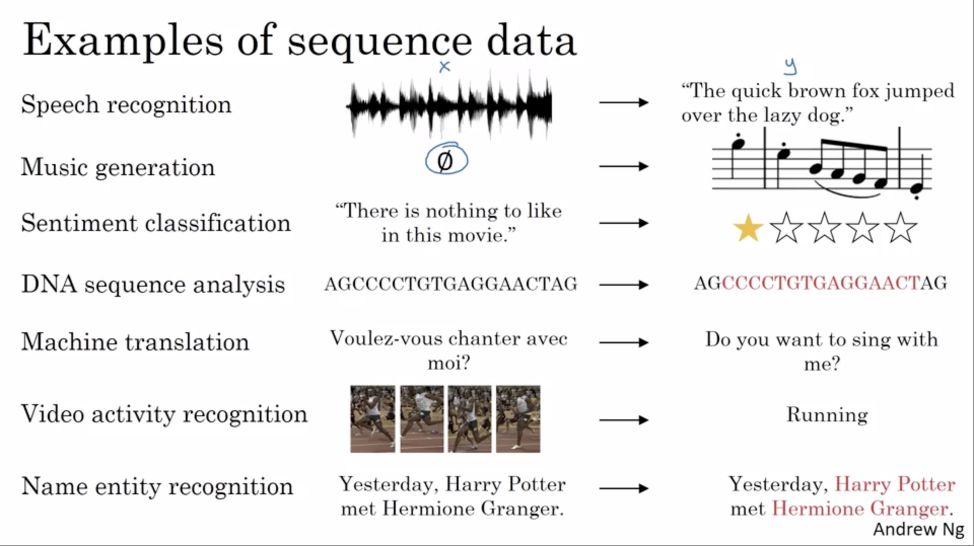
What are some other examples of sequential data? This screen shot from Andrew Ng’s lecture provide us with some common examples. The column in the middle are example inputs, and the column on the right are outputs that we might be potentially interested in generating from the inputs.

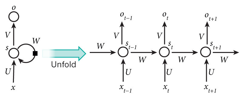
Notice that a common feature is that, there is no pre-determined requirements on the dimension of the input; we could be translating a sentence of 10 wrods, but we could also be translating a sentence of 20 words. This feature results from the structure of RNNs as shown below, where the analytical unit is reused, and could be unfolded into a network of variable length. This diagram also indicates that the output from the previous unit is processed as an input in the next unit, enabling the internal memory structure mentioned earlier.

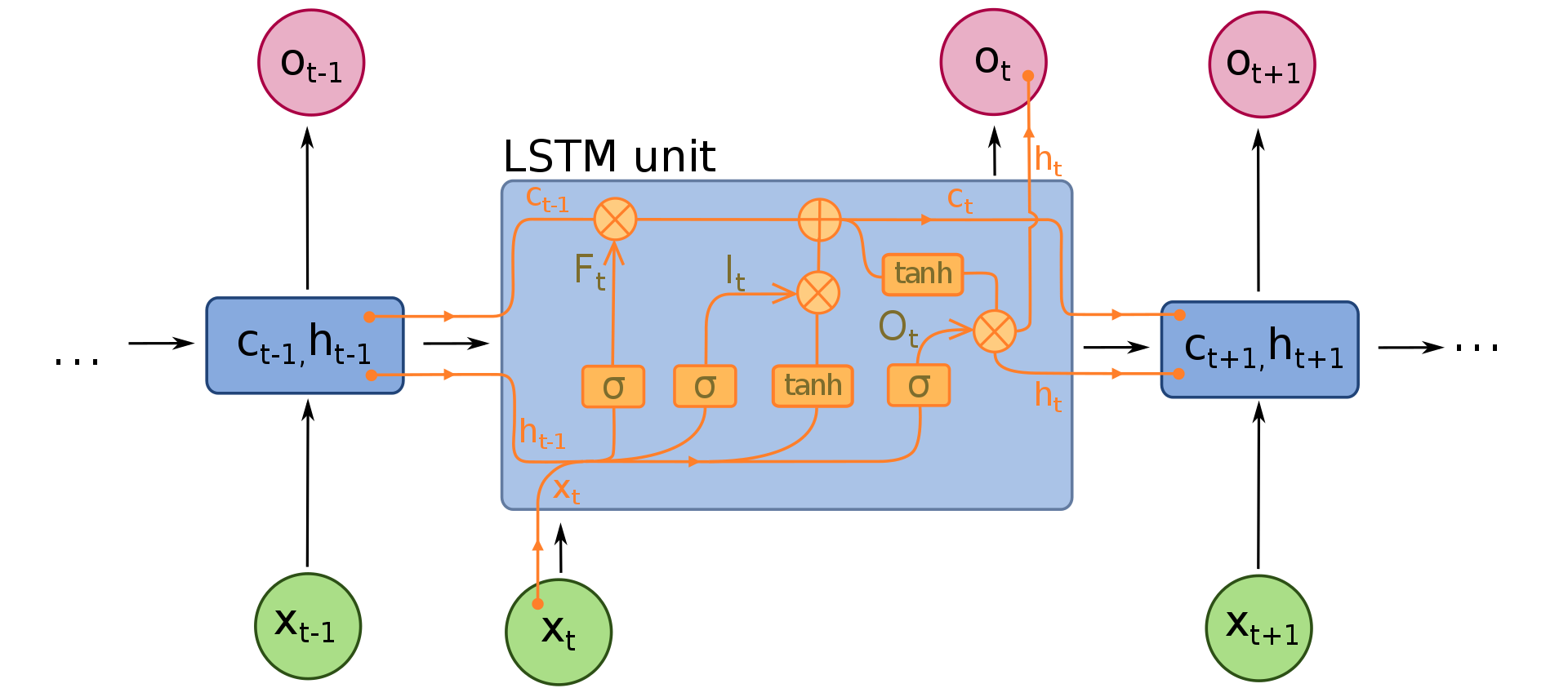
Each unit within the chain can be quite complicated; in fact, the diagram below shows the inner workings of an LSTM model. Given the variable and often long chain of networks, one can imagine many challenges RNNs could face when trying to implement backpropagation as seen in CNNs - for example, a same factor would commonly be multiplied by itself n (= # of time steps) times in various operations, leading to either vanishing (factor < 1) or exploding (factor > 1) results. In order to address this, a special gate, “forget” gate, is implemented in LSTM networks to ensure backpropagation can flow through an indefinite number of time steps, and that a significant event from many time steps ago, can still affect output on any given step. More details will be discussed in a blog post dedicated to RNNs.

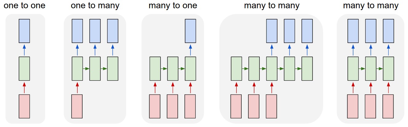
Finally, we will conclude with a high level overview of RNN structures. As illustrated below, a network can be categorized as one-to-one, one-to-many, many-to-one, and many-to-many.

1. one-to-one: RNNs are usually not of this specific format - on the contrary, CNNs such as image classifications do fall into this category. The input is one fixed-size image, and the output is a label / classification;
2. one-to-many: Image captioning, where input is an image, and output is vairable length text;
3. many-to-one: Sentiment analysis, where we can try to categorize reviews or comments into a specific category.
4. many-to-many: Two types of such networks are given, where the first one would correspond to tasks like language translation, and the second would entail real-time input and output, namely, tasks that do not wait for all inputs to arrive before start generating outputs. Such tasks include streaming video analysis that generates an output for each frame, but the output is also dependent on earlier frames (unlike plain CNNs).

(source)

That’s it! In conclusion, we have introduced the most common Deep Neural Networks out in the wild, namely, Convolutional Neural Networks, and Recurrent Neural Networks. We have discussed their use cases and basic structures, but you might be wondering to learn more about their inner workings - and that is exactly what we will bring to you in the next post.

Resources