

XGBoost - Gradient Boost
Links to Other Parts of Series
Prerequisites
Overview
If you’re not familiar with Decision Trees, Random Forests, and / or AdaBoost, and haven’t already checked out the blog posts linked above, please check that out first before proceeding with this post on Gradient Boost, since this does build upon the former posts.
Now that we got that covered, let’s dive right in!
What is Gradient Boost?
Gradient Boost is …
Gradient boosting is a machine learning technique for regression and classification problems, which produces a prediction model in the form of an ensemble of weak prediction models, typically decision trees. It builds the model in a stage-wise fashion like other boosting methods do, and it generalizes them by allowing optimization of an arbitrary differentiable loss function
In some sense, AdaBoost can be viewed as a special case of the general Gradient Boosting algorithms, but in common applications, they are quite different indeed. They are similar in that they both construct a series of trees (usually shallow ones) and make an ensemble out of them, but while AdaBoost does so by explicitly setting higher weights for previously misclassified samples, Gradient Boost uses the gradient to nudge the predictions towards the true values. While AdaBoost may be more intuitive to understand, without referencing concepts such as gradients, Gradient Boost are more flexible, and can be modified to work with a variety of loss functions, as long as their gradient is well behanved.
Steps
We will base our discussion off of the steps listed below:
|
|---|
| (source: Gradient boosting - Wikipedia) |
Here, x will be the input features (think height, weight, gender, etc.), and y will be the target variable (say, health index). Each subscription i would denote a sample from our data set. For Loss Function L(y, F(x)), which takes the true value y and the predicted value from x F(x), we will use a particular (but very commonly used) Loss Function: the MSE, Mean Squared Errors, which is the sum of the squared differences / errors between true and predicted values.
1. Initialization
The first step is to initialize some predictions (common for all samples, since gamma here is independent of i) in a reasonable fashion - here we specify the gamma to be the one to minimize our Cost (sum of losses). If we use MSE as our Loss function, it is easy to derive that the initial gamma = F0(x) = average of all y's:
To minimize SUM (y_i - gamma)^2 with respect to gamma, we take the derivative, and set it to 0, which leads us to SUM (y_i - gamma) = 0, so that SUM gamma's = SUM (y_i), where SUM gamma's = # of y_i's * gamma, and that leads to gamma = SUM (y_i) / (# of y_i's) = averages of y_i's.
2/a. Computing “pseudo-residuals”
Here in step 2, we are in an iteration for each tree we plan to constrcut (as the formula specifies, we plan to construct M trees to make up our eventual ensemble).
The pseudo-residual is defined as the partial derivatives of our Loss function (with respect to our prediction F) evaluated at our previous prediction. For our MSE loss function, and take our first iteration and first sample for example (m=1, i=1), we have:r_11 = F(x_1) - y_1, where we have set F(x_1) = F0(x_1) = average of y_i's. This is not that different from the residuals we are used to, but particularly because we have chosen the MSE as the loss function. The crucial part here is to recognize this as a Gradient, but which just happens to have an intuitive meaning.
2/b. Fit a weak learnner to the residuals
This step is usually a standard DT training, but where we can specify the depth and leaves we want the trees to have. Usually it is quite a shallow tree, since we will train M = quite large number of trees anyway.
2/c. Compute a tree-specific learning rate
The Wiki steps stated the general term of multiplier, but it is essentially our learning rate. To pick this learning rate, we try to solve another optimization problem, where we choose the learning rate that results in the least cost when taking into consideration the newly constructed tree.
2/d. Update the Model
Now we simply append our new tree to our existing model, multiplied by the optimal learning rate as specified in the previous step.
Loop
We perform steps 2/a to 2/d for each tree we want to construct, and our final output would be the initial guess F0, modified by a series of Decision Trees, each with a specific learning rate.
Why does it work?
It doesn’t seem hard to grasp the mechanical steps to perform such an algorithm, but intuitively, why does it work? In some sense, it is not that different from AdaBoost - in each step, we are focusing more on the “residuals”, the part that our previous model was not able to effectively account for, similarly to adding more weights to misclassified samples in AdaBoost. The animation below might provide some further insights:
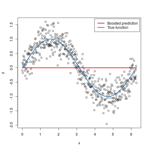
|
|---|
| (source: Gradient Boosting Machines - UC Business Analytics R Programming Guide) |
Here we are observing the model going through each iteration. Starting from a single horizontal line, we have predicted F0, something like the average’s of y_i’s. With each additional tree being added, a new vertical line is being displayed, and a shift in the prediction modified by the newly added tree. With more and more trees being added, our prediction is looking more and more like the True function.
Overfitting?
We might worry about overfitting, although ensemble models are in general better off in this regard, in practice Gradient Boosting still suffers from overfitting. There are quite a few things to tune during cross-validation steps in regards to that. For example, we can add shrinkage on the learning rate, so that each individual trees contribute less to the output. For more discussion on overfitting, I would recommend this article which goes into quite some details.
Afterthoughts
For those of you familiar with gradient descent, the whole gradient boosting thing might look familiar to you. So what is special about Gradient Boosting? This wonderful resource, Gradient boosting: frequently asked questions, makes a clear and concise summary:
Gradient descent optimization in the machine learning world is typically used to find the parameters associated with a single model that optimizes some loss function, such as the squared error. In other words, we are moving parameter vector around, looking for a minimal value of loss function that compares the model output for to the intended target.
In contrast, GBMs are meta-models consisting of multiple weak models whose output is added together to get an overall prediction. GBMs shift the current prediction […] around hoping to nudge it to the true target. The gradient descent optimization occurs on the output of the model and not the parameters of the weak models.
Getting a GBM’s approximation to is easy mathematically. Just add the residual to the current approximation. Rather than directly adding a residual to the current approximation, however, GBMs add a weak model’s approximation of the residual vector to the current approximation. By combining the output of a bunch of noisy models, the hope is to get a model that is much stronger but also one that does not overfit the original data. This approach is similar to what’s going on in Random Forests.
In some sense, Gradient Boosting is performing gradient descent in the function space of our prediction functions.
Conclusion
We are now finally well-prepared and ready for our end game - XGBoost. Tune in for our next post on the popular machine learning algorithm, and learn about the theories and applications, explained clearly!

Leave a comment