Neural Networks - 6. Convolutional Neural Networks: Case Studies (2)

Links to Other Parts of Series

• Neural Network Series

Overview

In the last post in our Neural Network series, we have looked into a few landmark Convolutional Neural Networks, including VGG, GoogLeNet/Inception, ResNet, and Wide ResNet. In this post, we will continue to study more recent networks, including DenseNet, Squeeze-and-Excitation Networks, and EfficientNet. It will follow the same structure as before, so let’s get right into it!

Networks

DenseNet

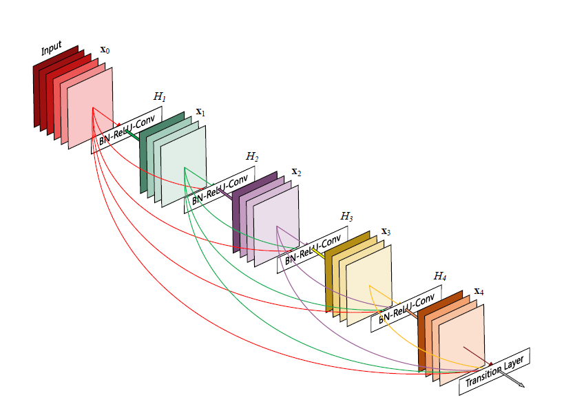
As we have seen from ResNet and other networks, having shorter, more efficient connections between layers may help the flow of information throughout the network, alleviating the issue of vanishing gradients. For example, ResNets and Highway Networks implement identity connections to pass signals skipping layers. How would it be like, if we instead connect all layers to all other layers? The result is the so called DenseNet, illustrated in the figure below.

Structure

(source: [1])

As we can see, each layer takes the outputs of previous layers as inputs, and passes on its own output to all subsequent layers.

(source: [1])

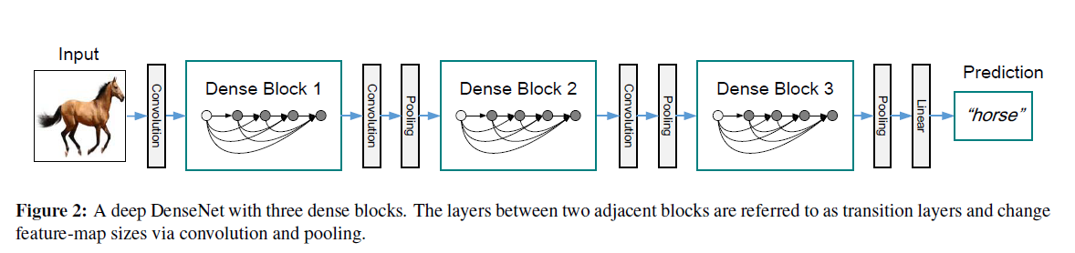
As we will explain later, the typical DenseNet is made up of Dense Blocks shown above, since within each block, the dimensions are kept the same for the ease of concatenating input/outputs from various layers. At the same time, we do want to keep reducing dimensions as we go deeper into the network, and hence the dense block structures.

Points of Interest

1. Possibly a bit counter-intuitive, but the dense connectivity pattern actually requires fewer parameters than comparable usual networks. That is because, we are directly passing in the state of the previous layers into the current layer, so there is no redundant feature maps to learn.
2. This is as opposed to ResNet, where each layer attempts to learn or re-learn all the information that is required to pass on to the deeper layers - DenseNet “explicitly differentiates between information that is added to the network and information that is preserved”, where it uses very narrow layers, so each layer is only adding “a small set of feature-maps to the collective knowledge of the network”. This feature-reusing results in fewer parameters to learn and train, and better parameter efficiency.
3. Aside from the imrpoved efficiency, DenseNet’s architecture also improves the flow of information and gradient, since each layer has direct access to the gradient of the loss function as well as the input layer. This improvement in information flow essentially makes the model easier and faster to train.
4. As mentioned above, DenseNet makes use of multiple densely connected dense blocks, since feature-map dimensions cannot change for the concatenation to work properly. To achieve the usual down-sampling effect in CNNs, transition layers consisting of batch normalization, convolutions and poolings are placed between dense blocks.
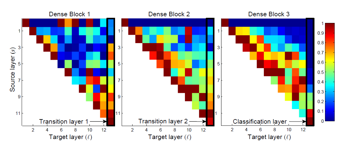
5. Since all previous layers’ outputs are concatenated into a single input for a particular layer, if each layer has k feature maps, then layer l would have k_0 + k x (l-1) input feature-maps, where k_0 is the original input dimension. The authors named k as the “growth rate” of the network, and demonstrated that even very narrow layers (e.g. k=12) can produce very good results, reassuring the parameter efficiency of the network.
6. A final note on feature reuse: To demonstrate that this is really happenning, the authors plotted the weights on the various layers of inputs in a trained network, as shown below.

(source: [1])

Take the block on the left (Dense Block 1) for example. The right-most column displays how it is weighting the inputs from each previous layers, and similarly for other columns. We see that although there are some variations, the weights are indeed spread over many input layers, indicating that even ver yearly layers are still being directly used in the deeper layers. On the other hand, if we look at the right-most column in the right-most block (the classification layer), we notice that the weights are concentrated on the last few layers. The authors suggest that this could indicate that some more high-level features are produced late in the network.

Squeeze-and-Excitation Networks

Most networks we’ve discussed up to this point has been focusing on facilitating information flow between layers, where the channels and filters haven’t really received much attention. In this Squeeze-and-Excitation Network (SENet) paper, the authors will focus on improving information efficiency through information sharing across layers, explicitly modelling channel interdependencies. By replacing standard convolutional layers with its SE block counterparts, they have imrpoved upon the state of the art (at that time) models and achieved first place in ILSVRC 2017.

Structure

(source: [2])

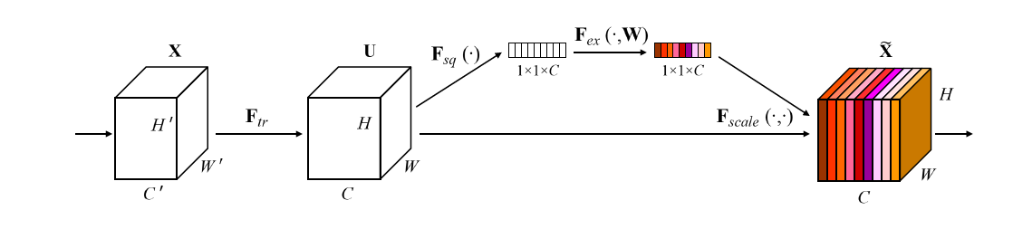
The main idea of SENets is to use the so-called SE Blocks to recalibrate the standard feature map output before passing it into the next layer. Take X as the input, put it through a transformation (F_tr) such as a convolution, which outputs the ordinary feature-map U. Now, instead of passing U into the next layer as usual, SE Block takes this U, and puts it through a squeeze operation (F_sq), an excitation operation (F_ex), then uses the result as a scaling factor, which operates on U, generating the recalibrated output. Let us take a closer look at the squeeze operator, and the excitation operator.

Squeeze

The squeeze operator is essentially a “global” averate pooling, a channel-wise statistics generated by “shrinking U through its spatial dimensions HxW”. If we call this statistics z, it would be a C dimensional vector, where C is the number of channels. That is, for each channel of the feature map, we would calculate the average valus in this channel, and put it in z. The resulting 1x1xC vector z is the result as seen in the figure above, after the F_sq operator.

Excitation

The excitation layer aims to make use of this z vector. The excitation layer can be broekn down into 3 smaller parts - a FC layer that reduces dimensionality to C/r (recall Inception Modules), then a ReLU operation, then another FC layer to recover the dimension to C, and finally a sigmoid activation function before generating the output. In terms of the figure above, the output here is the 1x1xC vector with colored stripes, after the F_ex operator.

Recalibration

The final step is to recalibrate U with the output of F_ex, that is done by simply rescaling U channel-wise by the 1x1xC vector, as illustrated in the figure above.

Points of Interest

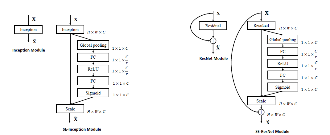(source: [2])

1. The SE block can be easily integrated into standard architecture. For example, the figure above illustrates integrating SE blocks in Inception modules and ResNet, respectively.

2. Computational efficiency: SENets do not introduce much computational overhead, but improves the performance of existing networks a lot. For example, if applied to standard ResNet-50, SE-ResNet-50 increases the GFLOPS (think operations) by 0.26%, but improves the accuracy of ResNet-50 to the point of approaching ResNet-101, which requires much larger GFLOPS.

3. In terms of parameters, SE blocks introduce more parameters only in the two FC layers within the excitation operation. Still using the ResNet-50 example, the corresponding SE-ResNet-50 introduces a 10% increase in parameters. In practice, the majority of these parameters come from the final layers of the network (where we have more channels hence larger C’s). The authors experimented with dropping the final SE blocks, and was able to reduce the parameters to only a 4% increase without losing much accuracy.

4. In line with this observation, the authors also explored the role of excitations. The method is by studying the distribution of excitations for a few distinct classes (in particular, goldfish, pug, plane, and cliff). In the final stages, the SE blocks become saturated with most of the activations close to one, which makes them closer to an identity mapping, and less improtant in accuracy. Other findings along the way are also consistent with ealier studies, where earlier layers display a similar distribution across classes, while deeper layers’ activations are much more class-specific.

EfficientNet

There have been a variety of ways to scale up a model / network in an attempt to achieve higher accuracy, but the scaling has either been rather one-dimensional (in depth / width, or image resolution), or tediously manual. In this EfficientNet paper, the authors propsed a simple “Compound Scaling” rule, and demonstrated its effectiveness. In essence, it renders a balanced scaling method, where the depth, width and resolution scale together. Intuitively, this makes sense, since if input image is bigger, more layers and channels would be required to capture the fine-grained patterns. Additionally, empirical evidence has suggested that scaling up single dimension does work, but the effect diminishes quickly. Let’s take a look at the idea of EfficentNet.

Structure

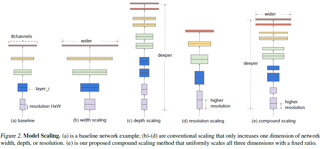
(source: [3])

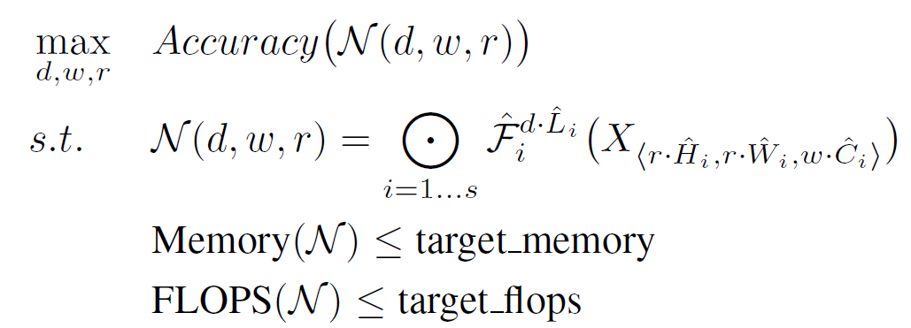
As opposed to focusing on one-dimensional scaling as we often see, EfficientNet proposes the compound scaling illustrated above. The idea is acutally super simple. If we model the network as a collection of convolutional layers F operators, we can parameterize a given, predefined network structure’s optimization problem by the following equation:

(source: [3])

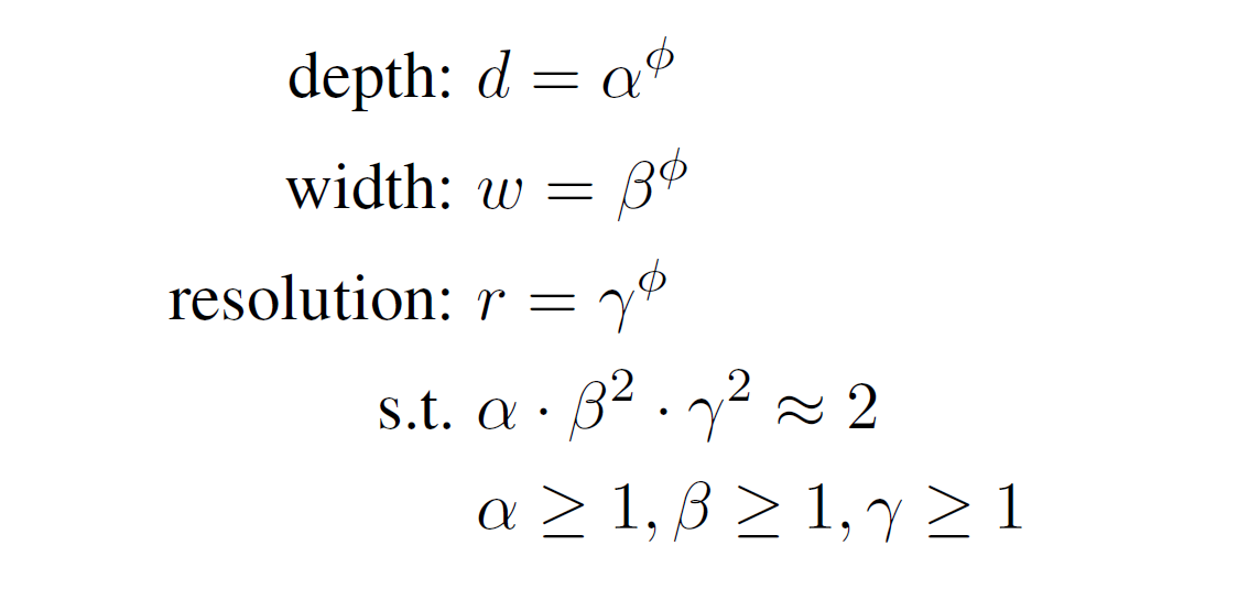
Here, d, w, and r are the scaling factors, X is the input to each layer F, whrer H, W, and C represent the input dimensions. Superscipts on F represents the depth of the network. In summary, and in plain words, our goal is to maximize accuracy of the network by choosing the caling factors, subject to the memory and FLOP (operations) constraints. Now in particular for the proposed Compound Scaling, we further constrain d, w, and r to the following conditions:

(source: [3])

Where Φ is a user specified coefficient to control how much resource to use. The particular structure of the constraint on a x b^2 x γ^2 = 2 is reflective of the fact that in a regular conv network, FLOPS is proportional to d, w^2, and r^2 respectively. Now that the problem is formulated, we just need to do a grid search over the constrained space, and find the optimal values for the scaling factors. In practice, doing this grid search on a large model is still prohibitively expensive, so the authors performed 2-step optimization: first optimizing on a smaller model, then with the optimal a, b and γ found in the small model, scale up the model through Φ.

Points of Interest

1. If we plot out the Accuracy-FLOPS curve for EfficientNet and other ConvNets (below), we can see that EfficientNet models achieve better accuracy with much fewer FLOPS. In particular, “EfficientNet-B3 achieves higher accuracy than ResNeXt-101 using 18x fewer FLOPS”.

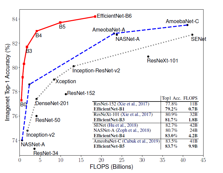
   (source: [3])

2. The plot below compares the class activation map for a few models scaled differently. Recall that a class activation map to some sense illustrates what the particular layer is detecting. We can see that EfficientNet model with compound scaling (right-most) is able to “focus on more relevant regions with more object details, while other models [single dimension scaling or comparable computation level] are either lack of object details or unable to capture all objects in the images.”

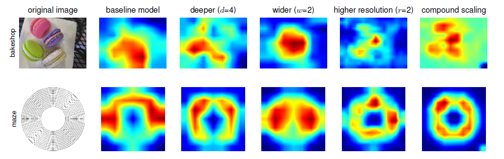
   (source: [3])

Conclusion

In this post we have reviewed a few more recent neural networks, and we see that instead of blindly building deeper and deeper networks, people are exploring ways to design more efficient network structures, often making some improvements that could be applied to a variety of existing networks, and making them perform better. understanding and keeping these structure modifications in mind could prove very beneficial when it comes to designing your own network, as they could often be dropped in to replace standard structures, and improve your network performance.

Resources

References:

[1] Huang, Gao, et al. “Densely connected convolutional networks.” Proceedings of the IEEE conference on computer vision and pattern recognition. 2017.

[2] Hu, Jie, Li Shen, and Gang Sun. “Squeeze-and-excitation networks.” Proceedings of the IEEE conference on computer vision and pattern recognition. 2018.

[3] Tan, Mingxing, and Quoc V. Le. “EfficientNet: Rethinking Model Scaling for Convolutional Neural Networks.” arXiv preprint arXiv:1905.11946 (2019).