

Neural Networks - 7. Convolutional Neural Networks: Example with Kaggle Challenge
Links to Other Parts of Series
Overview
In the last 2 post in our Neural Network series, we have looked into a few landmark Convolutional Neural Networks, including VGG, GoogLeNet/Inception, ResNet, Wide ResNet, DenseNet, SENets, and EfficientNet. In this post, we will try to take some ideas from these networks, and implement some codes to paly around a Kaggle challenge from the past. We will not be particularly trying to achieve the absolute best result on the dataset, but to explore the end-to-end process, their implementations, as well as small tweaks here and there while observing their effects, with the ultimate goal of improving our understanding of neural networks in general.
Challenge Background
You can find more details on the background and the set up of the challenge on Kaggle, but the overall idea is to train a neural network that could tell the difference between 12 classes of fairly similar plants. As you might have discovered, there are plenty of publicly available kaggle notebooks sharing their implementations, and here in our post we will mainly be referencing the following ones:
- Seedlings - Pretrained keras models (notebook 1)
- Keras simple model (0.97103 Best Public Score) (notebook 2)
We will explain what they are doing in their implementations, and make modifications along the way. Ready? Let’s get started!
Exploration
The first thing we do when presented with a task is usually to explore the data a bit. For our example, we will check the distribution of our data, make some plots to visualize what we are dealing with, and go from there. To help you make sense with our code, the folder structure I have is as follows:
- project_root
    - data
        - test
            - image_1
            - image_2
            ...
        - train
            - Black-grass
                - image_1
                - image_2
                ...
            - Charlock
                - image_1
                - image_2
                ...

            ... more classes

    - models
        - <saved models / weights>

    - <notebooks / codes>
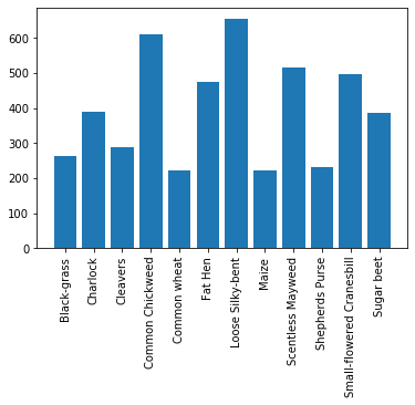
Data Distribution
To get an idea of training example distributions, we can checkout how many images are included in each class-specific folder.
import os
import numpy as np
import matplotlib.pyplot as plt

# TRAIN_IMG_PATH = /path/to/project_root/data/train
classes = {}
for class_name in os.listdir(TRAIN_IMG_PATH):
    classes[class_name] = len(os.listdir(os.path.join(TRAIN_IMG_PATH, class_name)))
print(classes)

########################
{'Black-grass': 263,
 'Charlock': 390,
 'Cleavers': 287,
 'Common Chickweed': 611,
 'Common wheat': 221,
 'Fat Hen': 475,
 'Loose Silky-bent': 654,
 'Maize': 221,
 'Scentless Mayweed': 516,
 'Shepherds Purse': 231,
 'Small-flowered Cranesbill': 496,
 'Sugar beet': 385}
Since we’re doing a blog, let’s get a tiny bit fancier and generate a bar plot:
plt.bar(classes.keys(), classes.values())
plt.xticks(rotation=90)
|
|---|
| (source: Code Above) |
As we can see, the number of images within each class ranges from 200 tojust above 600. The incalance is not too bad but with this in mind we could try to experiment with balancing dataset in mind later down the road.
Example Input
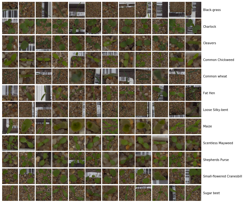
Now let’s take a look at how our inputs look like. This following block of code is adapted from notebook [1] above, which really comes in handy for exploring an image set.
from mpl_toolkits.axes_grid1 import ImageGrid
import numpy as np
import matplotlib.pyplot as plt
from keras.preprocessing import image
import pandas as pd

CATEGORIES = ['Black-grass', 'Charlock', 'Cleavers', 'Common Chickweed', 'Common wheat', 'Fat Hen', 'Loose Silky-bent',
              'Maize', 'Scentless Mayweed', 'Shepherds Purse', 'Small-flowered Cranesbill', 'Sugar beet']
NUM_CATEGORIES = len(CATEGORIES)

train = []
for category_id, category in enumerate(CATEGORIES):
    for file in os.listdir(os.path.join(TRAIN_IMG_PATH, category)):
        train.append(['train/{}/{}'.format(category, file), category_id, category])
train = pd.DataFrame(train, columns=['file', 'category_id', 'category'])


def read_img(filepath, size):
    img = image.load_img(os.path.join(DATA_PATH, filepath), target_size=size)
    img = image.img_to_array(img)
    return img


fig = plt.figure(1, figsize=(NUM_CATEGORIES, NUM_CATEGORIES))
grid = ImageGrid(fig, 111, nrows_ncols=(NUM_CATEGORIES, NUM_CATEGORIES), axes_pad=0.05)
i = 0
for category_id, category in enumerate(CATEGORIES):
    for filepath in train[train['category'] == category]['file'].values[:NUM_CATEGORIES]:
        ax = grid[i]
        img = read_img(filepath, (224, 224))
        ax.imshow(img / 255.)
        ax.axis('off')
        if i % NUM_CATEGORIES == NUM_CATEGORIES - 1:
            ax.text(250, 112, filepath.split('/')[1], verticalalignment='center')
        i += 1
plt.show()
This would generate the plot below:
 |
|---|
| (source: Code Above) |
As we can see, these plants’ images are fairly difficult to discern - as a human being, if I train myself on these images for a couple of hours, I’m really not sure if I can out perform the network we are about the build xD.
CNN Implementations
Now that we know what we’re dealing with, there are a couple of options in terms of our attack plan. One way is to start from a pre-trained model, make some tweaks here and there, then fine-tune the weights while training the model on our images. The other approach would be to build a network from the ground up, and train it from scratch. There are pros and cons to each approach, and both can work really well. For example, [notebook 1] above extracted features from the Xception net and used their pretrained weights, while [notebook 2] built a new network from scratch. We will start by exploring [notebook 2].
Option 1: Build from Scratch
I will refer you to the original notebook for the details, while I will provide some code snippets and explain what the codes are doing.
Step 1: Imports and Setup
First we import all the good stuffs Keras provide us with, and set up two dictionaries we would use in training and testing. A large part of the later codes, including img_reshape, fill_dict, reader, etc. are all helper functions to prepare the data and get them ready for training or testing models. It is beneficial to familiar yourself with such codes, as they can often be reused across various projects, depending on the structure of your training data. However, we will not go into the details here, but rather focus on the neural network itself.
Step 2: Define Building Blocks
# Dense layers set
def dense_set(inp_layer, n, activation, drop_rate=0.):
    dp = Dropout(drop_rate)(inp_layer)
    dns = Dense(n)(dp)
    bn = BatchNormalization(axis=-1)(dns)
    act = Activation(activation=activation)(bn)
    return act

# Conv. layers set
def conv_layer(feature_batch, feature_map, kernel_size=(3, 3),strides=(1,1), zp_flag=False):
    if zp_flag:
        zp = ZeroPadding2D((1,1))(feature_batch)
    else:
        zp = feature_batch
    conv = Conv2D(filters=feature_map, kernel_size=kernel_size, strides=strides)(zp)
    bn = BatchNormalization(axis=3)(conv)
    act = LeakyReLU(1/10)(bn)
    return act
Here the notebook defined 2 types of neural network blocks that will make up the final model. The usual convolutional layer which is made up of a (optional) padding operation, the usual Conv2D, followed by batch-normalization and a LeakyReLU activation. The dense layer, which are applied towards the end of the network, is prepended with a dropout operation, and then BN and a specifiable activation (which in our case, would be tanh and softmax for the last two layers.)
Step 3: Build the Model
def get_model():
    inp_img = Input(shape=(51, 51, 3))

    # 51
    conv1 = conv_layer(inp_img, 64, zp_flag=False)
    conv2 = conv_layer(conv1, 64, zp_flag=False)
    mp1 = MaxPooling2D(pool_size=(3, 3), strides=(2, 2))(conv2)
    # 23
    conv3 = conv_layer(mp1, 128, zp_flag=False)
    conv4 = conv_layer(conv3, 128, zp_flag=False)
    mp2 = MaxPooling2D(pool_size=(3, 3), strides=(2, 2))(conv4)
    # 9
    conv7 = conv_layer(mp2, 256, zp_flag=False)
    conv8 = conv_layer(conv7, 256, zp_flag=False)
    conv9 = conv_layer(conv8, 256, zp_flag=False)
    mp3 = MaxPooling2D(pool_size=(3, 3), strides=(2, 2))(conv9)
    # 1
    # dense layers
    flt = Flatten()(mp3)
    ds1 = dense_set(flt, 128, activation='tanh')
    out = dense_set(ds1, 12, activation='softmax')

    model = Model(inputs=inp_img, outputs=out)

    # The first 50 epochs are used by Adam opt.
    # Then 30 epochs are used by SGD opt.

    #mypotim = Adam(lr=2 * 1e-3, beta_1=0.9, beta_2=0.999, epsilon=1e-08)
    mypotim = SGD(lr=1 * 1e-1, momentum=0.9, nesterov=True)
    model.compile(loss='categorical_crossentropy',
                   optimizer=mypotim,
                   metrics=['accuracy'])
    model.summary()
    return model
Now we get to the exciting step (at least for me). Here we define a get_model function, which builds the model we would use for our CNN. We start with 51x51 input images, which is smaller than most of our original training images. This reduces the amount of computation required, but may lead to slightly poorer results. Then it is a series of conv layers stacked together, with MaxPooling layers in between, Towards the end, we flatten out the network, and switch to FC layers to perform the final classification, which is 12-dimensional as we have 12 classes.
Notice that the notebook added a comment to switch from Adam to SGD optimizer after 50 epochs; this is perhaps due to findings in [1], where they demonstrated that
Despite superior training outcomes, adaptive optimization methods such as Adam, Adagrad or RMSprop have been found to generalize poorly compared to Stochastic gradient descent (SGD). These methods tend to perform well in the initial portion of training but are outperformed by SGD at later stages of training.
Step 4: Train the Model
# MODEL_PATH = /path/to/project_root/models

def get_callbacks(filepath, patience=5):
    lr_reduce = ReduceLROnPlateau(monitor='val_accuracy', factor=0.1, epsilon=1e-5, patience=patience, verbose=1)
    msave = ModelCheckpoint(filepath, save_best_only=True)
    return [lr_reduce, msave]

def train_model(img, target):
    callbacks = get_callbacks(filepath=os.path.join(MODEL_PATH, 'model_weight_Adam.hdf5'), patience=6)
    gmodel = get_model()
    # When we start SGD rounds of training, we load weights from Adam trainings and proceed.
    # callbacks = get_callbacks(filepath=os.path.join(MODEL_PATH, 'model_weight_SGD.hdf5'), patience=6)
    # gmodel.load_weights(filepath=os.path.join(MODEL_PATH, 'model_weight_Adam.hdf5'))
    x_train, x_valid, y_train, y_valid = train_test_split(
                                                img,
                                                target,
                                                shuffle=True,
                                                train_size=0.8,
                                                random_state=RANDOM_STATE
                                            )
    gen = ImageDataGenerator(
            rotation_range=360.,
            width_shift_range=0.3,
            height_shift_range=0.3,
            zoom_range=0.3,
            horizontal_flip=True,
            vertical_flip=True
    )
    gmodel.fit_generator(gen.flow(x_train, y_train,batch_size=BATCH_SIZE),
               steps_per_epoch=10*len(x_train)/BATCH_SIZE,
               epochs=EPOCHS,
               verbose=1,
               shuffle=True,
               validation_data=(x_valid, y_valid),
               callbacks=callbacks)
Here we defined a callback, which is called upon after each epoch. The particular callback defiend here does 2 things: 1. If the validation accuracy starts to plateau, we reduce our learning rate to perform the final few epochs, and 2. Save the current weights, if it has achieved better results than earlier weights. Notice that just as with our optimizer, the we will specify slightly different models for the earlier and later part of the training. In particular, when we switch to SGD, we would want to load the weights as the result of the Adam training rounds, and proceed from there.
Step 5: Running it!
train_dict, test_dict = reader()
X_train = np.array(train_dict['image'])
y_train = to_categorical(np.array([CLASS[l] for l in train_dict['class']]))
train_model(X_train, y_train)
Here we invoke the helper functions, and pass the training set into the training model. Some print outs are pasted below, where we can see the accuracy on both the training and validation set has reached a fairly high level, and as the accuracy plateau, the callback reduced the learning rate after epoch 26. Notice that this is the 2nd round of training - we first do the Adam optimizer epochs, and when that is done, we tweak the model a bit as suggested in the code comments, and train for another 30 epochs.
...
...
Epoch 24/30
2375/2375 [==============================] - 356s 150ms/step - loss: 0.1010 - accuracy: 0.9661 - val_loss: 0.1378 - val_accuracy: 0.9411
Epoch 25/30
2375/2375 [==============================] - 356s 150ms/step - loss: 0.1017 - accuracy: 0.9664 - val_loss: 0.1141 - val_accuracy: 0.9568
Epoch 26/30
2375/2375 [==============================] - 356s 150ms/step - loss: 0.0979 - accuracy: 0.9671 - val_loss: 0.1304 - val_accuracy: 0.9474

Epoch 00026: ReduceLROnPlateau reducing learning rate to 2.0000000949949027e-05.
Epoch 27/30
2375/2375 [==============================] - 356s 150ms/step - loss: 0.0941 - accuracy: 0.9683 - val_loss: 0.1218 - val_accuracy: 0.9537
Epoch 28/30
2375/2375 [==============================] - 356s 150ms/step - loss: 0.0877 - accuracy: 0.9701 - val_loss: 0.1238 - val_accuracy: 0.9547
Epoch 29/30
2375/2375 [==============================] - 356s 150ms/step - loss: 0.0883 - accuracy: 0.9710 - val_loss: 0.1276 - val_accuracy: 0.9526
Epoch 30/30
2375/2375 [==============================] - 356s 150ms/step - loss: 0.0922 - accuracy: 0.9689 - val_loss: 0.1232 - val_accuracy: 0.9547
Option 2: Use Pre-trained Networks
I will again refer you to the original notebook for the details. Here we will talk about just a few interesting points about this particular transfer learning application.
Extracting the Model
xception_bottleneck = xception.Xception(weights='imagenet', include_top=False, pooling=POOLING)
train_x_bf = xception_bottleneck.predict(Xtr, batch_size=32, verbose=1)
valid_x_bf = xception_bottleneck.predict(Xv, batch_size=32, verbose=1)
Here, xception_bottleneck loads the pre-trained model with weights that were obtained on imagenet. include_top is set to False, which excludes the finaly classification layer. This is often the case, since for different applications, the output layer would most likely differ. Here in our case, we have 12 classes to differentiate, so the output layer could be a 1x12 layer. Sometimes we append such a layer to the loaded model, but then we would need to further train our model to fine-tune the parameters in the last layers.
Logistic Regression as the Last Layer
Instead of appending a dense layer as the output, what this notebook did was totake the output from xception_bottleneck, which is 1x2048 in size, and project that output onto a LogisticRegression model.
# LogReg on Xception bottleneck features
logreg = LogisticRegression(multi_class='multinomial', solver='lbfgs', random_state=SEED, max_iter=1000)
logreg.fit(train_x_bf, ytr)
valid_probs = logreg.predict_proba(valid_x_bf)
valid_preds = logreg.predict(valid_x_bf)
print('Validation Xception Accuracy {}'.format(accuracy_score(yv, valid_preds)))
Here train_x_bf is the output from xception_bottleneck.predict(Xtr, batch_size=32, verbose=1), which is a set of 1x2048 arrays representing whatever features the Xception model has abstracted from each of the input images, meaning that train_x_bf has dimension of # of training images x 2048. logreg.fit(train_x_bf, ytr) then fits the logistic regression with the training data, which essentially takes the 1x2048 input and produces a prediction about which class this input belongs to. In some sense, the Xception model acted as a feature-extraction black-box, which extracts 2048 features from an input image, and the Logistic model simply makes predictions based on the extracted features.
Confusion Matrix
Another thing to take away from this notebook is a helpful block of code to produce a confusion matrix.
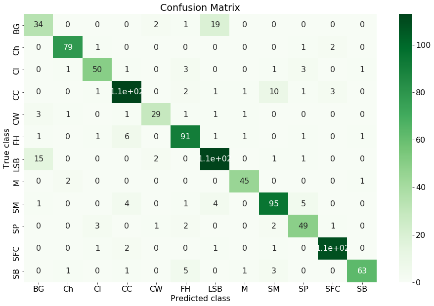 |
|---|
| (source: Produced by Code from [notebook 2]) |
Values on the diagonal are GOOD - that means for an image of class X, we have indeed predicted class X. Off-diagonal values represents incorrect predictions. For example, take the 19 on the first row. That value means for 19 of BG plants, we have misclassified them as LSB plants. Confusion matrix can often help us understand the detailed performance of our model - instead of a blanket number of 86% accuracy rate, we can tell from the Confusion matrix that our model is having difficulty telling BG and LSB apart (also notice the 15 in first column).
Comparisons
For our Option 2, pre-trained method, the output on the validation set is Validation Xception Accuracy 0.8639523336643495, which is not super high, but surprisingly decent, since we need to remember that we have not done any training on the CNN layers - we simply loaded pre-trained weights (which has been trained on ImageNet, instead of these plant images), and fitted a Logistic regression. The whole process took me less than 10 minutes, while the training of the model from scratch took me overnight.
In light of these, some additional trainings are often performed on pre-trained models. For example, as mentioned earlier, we could append a dense layer to the Xception model, and selectively freeze/unfreeze some layers to train. Usually lower level layers are fine to leave as is, since we believe they are detecting features that are fairly common across data sets; on the other hand, deeper layers might be detecting task-specific features, and it might be worth training and fine-tuning some weights in those layers to improve performance.
All in all, this blog post just shows how readily available the tools for Deep Learning are available to us, and how “easily” it is to create some models that are achieving very good results. I put “easy” in quotes, since there is no doubt that there had been a lot of trials and errors, along with tinkering and experimentation with layers / dimensions / optimization functions / etc. before [notebook 1] was able to determine which hyperparameters works well, but the bottom line is, the more you practice and work on real projects, the better intuition you will have in terms of what to choose for each task presented.
Resources

References
[1] Keskar, Nitish Shirish, and Richard Socher. “Improving generalization performance by switching from adam to sgd.” arXiv preprint arXiv:1712.07628 (2017).
Leave a comment